Technologies for Computational Science Boyana Norris Argonne National

Technologies for Computational Science Boyana Norris Argonne National Laboratory http: //www. mcs. anl. gov/~norris March 15, 2005

Outline n Automatic differentiation ¨ Applications in optimization ¨ How AD works n n n Components for scientific computing Performance evaluation and modeling Bringing it all together March 15, 2005 2

What is automatic differentiation? Automatic Differentiation (AD): a technology for automatically augmenting computer programs, including arbitrarily complex simulations, with statements for the computation of derivatives, also known as sensitivities. The Computational Differentiation Project at Argonne National Laboratory March 15, 2005 3

What is it good for? n The need to accurately and efficiently compute derivatives of complicated simulation codes arises regularly in ¨ Optimization (finding a minimum) ¨ Solving nonlinear differential equations ¨ Sensitivity and uncertainty analysis ¨ Inverse Problems, including: n n n Data assimilation Parameter identification AD tools automate the generation of derivative code without precluding the exploitation of highlevel knowledge. March 15, 2005 4

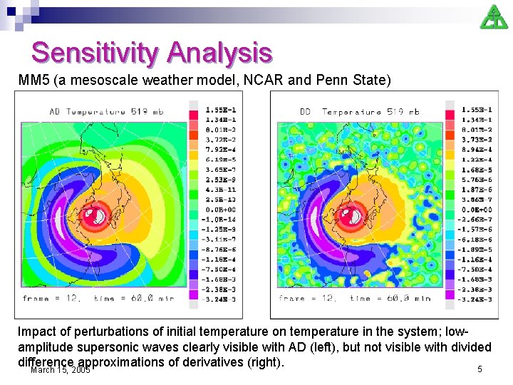
Sensitivity Analysis MM 5 (a mesoscale weather model, NCAR and Penn State) Impact of perturbations of initial temperature on temperature in the system; lowamplitude supersonic waves clearly visible with AD (left), but not visible with divided difference approximations of derivatives (right). 5 March 15, 2005

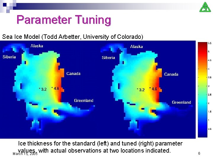
Parameter Tuning Sea Ice Model (Todd Arbetter, University of Colorado) Ice thickness for the standard (left) and tuned (right) parameter values, with actual observations at two locations indicated. March 15, 2005 6

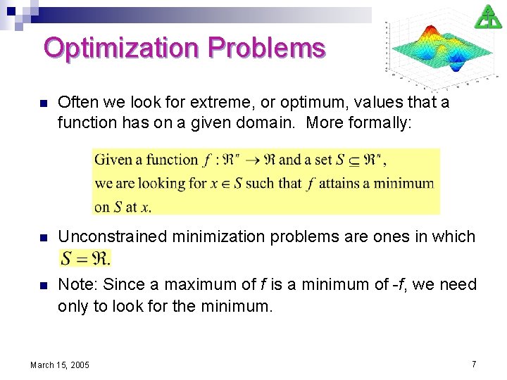
Optimization Problems n Often we look for extreme, or optimum, values that a function has on a given domain. More formally: n Unconstrained minimization problems are ones in which n Note: Since a maximum of f is a minimum of -f, we need only to look for the minimum. March 15, 2005 7

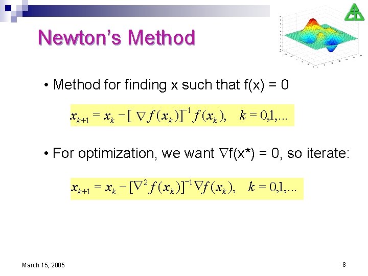
Newton’s Method • Method for finding x such that f(x) = 0 -1 = xk +1 xk [ f ( x k )] f ( xk ), k = 0, 1, . . . • For optimization, we want f(x*) = 0, so iterate: xk +1 = xk - [ 2 f ( x k )] 1 f ( xk ), k = 0, 1, . . . March 15, 2005 8

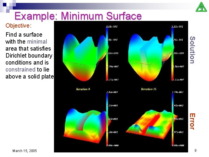
Example: Minimum Surface Objective: Solution Find a surface with the minimal area that satisfies Dirichlet boundary conditions and is constrained to lie above a solid plate. Error March 15, 2005 9

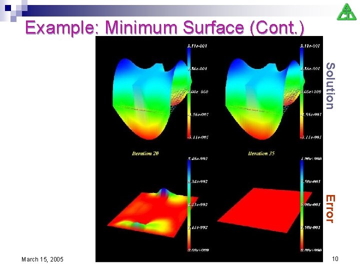
Example: Minimum Surface (Cont. ) Solution Error March 15, 2005 10

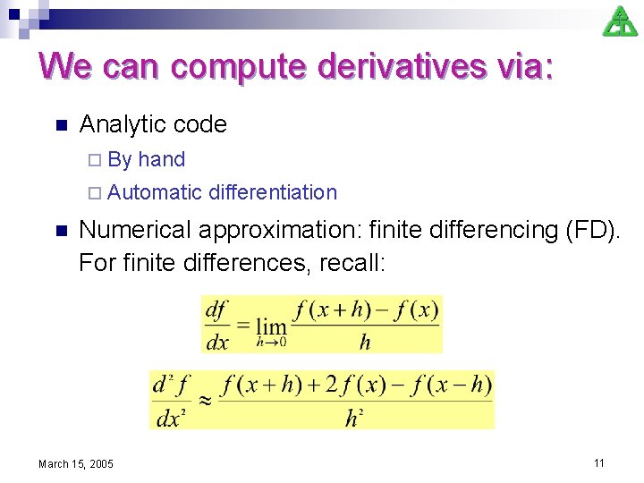
We can compute derivatives via: n Analytic code ¨ By hand ¨ Automatic n differentiation Numerical approximation: finite differencing (FD). For finite differences, recall: March 15, 2005 11

Why use AD? n Compared with other methods (numerical differentiation via finite differences, hand coding, etc. ), AD offers a number of advantages: ¨ Accuracy ¨ Performance ¨ Reduced effort ¨ Algorithm-awareness March 15, 2005 12

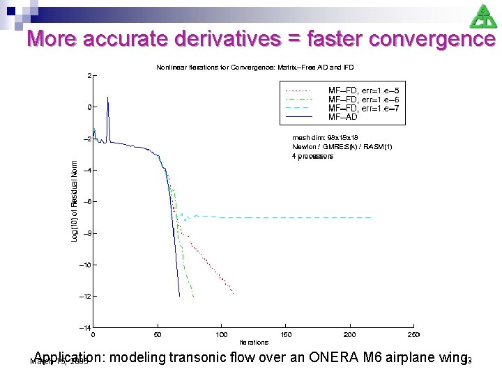
More accurate derivatives = faster convergence Application: modeling transonic flow over an ONERA M 6 airplane wing. 13 March 15, 2005

Who uses it? AD has been successfully employed in applications in: n Atmospheric chemistry n Breast cancer modeling n Computational fluid dynamics n Mesoscale climate modeling n Network Enabled Optimization System n Semiconductor device modeling n And also: groundwater remediation, multidisciplinary design optimization, reactor engineering, superconductor simulation, multibody simulations, molecular dynamics simulations, power system analysis, water reservoir simulation, and storm modeling. March 15, 2005 14

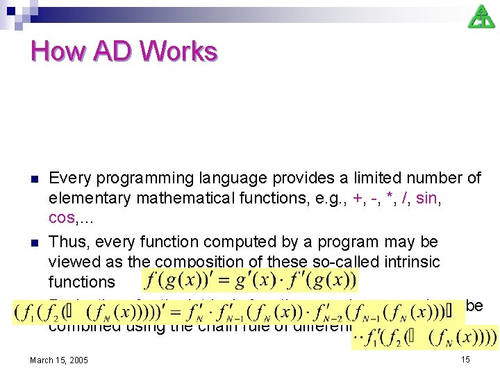
How AD Works n n n Every programming language provides a limited number of elementary mathematical functions, e. g. , +, -, *, /, sin, cos, … Thus, every function computed by a program may be viewed as the composition of these so-called intrinsic functions Derivatives for the intrinsic functions are known and can be combined using the chain rule of differential calculus March 15, 2005 15

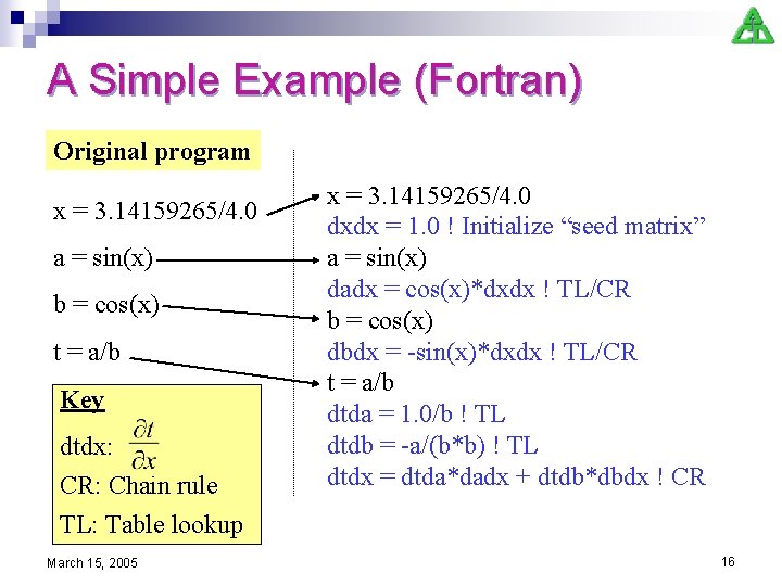
A Simple Example (Fortran) Original program x = 3. 14159265/4. 0 a = sin(x) b = cos(x) t = a/b Key dtdx: CR: Chain rule TL: Table lookup March 15, 2005 Differentiated program x = 3. 14159265/4. 0 dxdx = 1. 0 ! Initialize “seed matrix” a = sin(x) dadx = cos(x)*dxdx ! TL/CR b = cos(x) dbdx = -sin(x)*dxdx ! TL/CR t = a/b dtda = 1. 0/b ! TL dtdb = -a/(b*b) ! TL dtdx = dtda*dadx + dtdb*dbdx ! CR 16

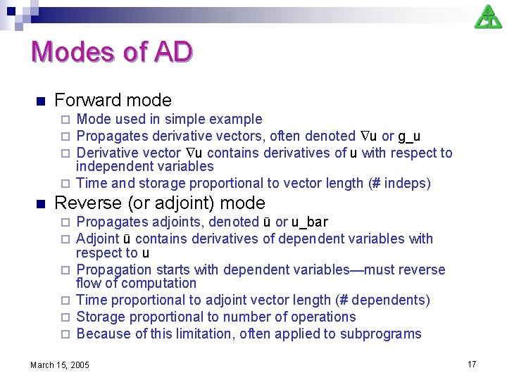
Modes of AD n Forward mode Mode used in simple example Propagates derivative vectors, often denoted u or g_u Derivative vector u contains derivatives of u with respect to independent variables ¨ Time and storage proportional to vector length (# indeps) ¨ ¨ ¨ n Reverse (or adjoint) mode ¨ ¨ ¨ Propagates adjoints, denoted ū or u_bar Adjoint ū contains derivatives of dependent variables with respect to u Propagation starts with dependent variables—must reverse flow of computation Time proportional to adjoint vector length (# dependents) Storage proportional to number of operations Because of this limitation, often applied to subprograms March 15, 2005 17

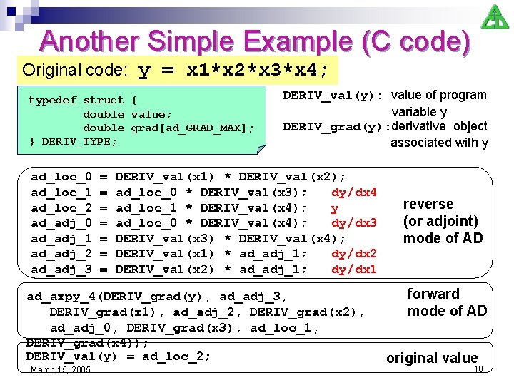
Another Simple Example (C code) Original code: y = x 1*x 2*x 3*x 4; typedef struct { double value; double grad[ad_GRAD_MAX]; } DERIV_TYPE; ad_loc_0 ad_loc_1 ad_loc_2 ad_adj_0 ad_adj_1 ad_adj_2 ad_adj_3 = = = = DERIV_val(y): value of program variable y DERIV_grad(y): derivative object associated with y DERIV_val(x 1) * DERIV_val(x 2); ad_loc_0 * DERIV_val(x 3); dy/dx 4 ad_loc_1 * DERIV_val(x 4); y ad_loc_0 * DERIV_val(x 4); dy/dx 3 DERIV_val(x 3) * DERIV_val(x 4); DERIV_val(x 1) * ad_adj_1; dy/dx 2 DERIV_val(x 2) * ad_adj_1; dy/dx 1 ad_axpy_4(DERIV_grad(y), ad_adj_3, DERIV_grad(x 1), ad_adj_2, DERIV_grad(x 2), ad_adj_0, DERIV_grad(x 3), ad_loc_1, DERIV_grad(x 4)); DERIV_val(y) = ad_loc_2; March 15, 2005 reverse (or adjoint) mode of AD forward mode of AD original value 18

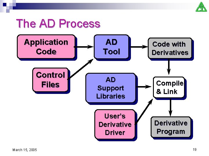
The AD Process Application Code Control Files AD Tool Code with Derivatives AD Support Libraries Compile & Link User’s Derivative Driver March 15, 2005 Derivative Program 19

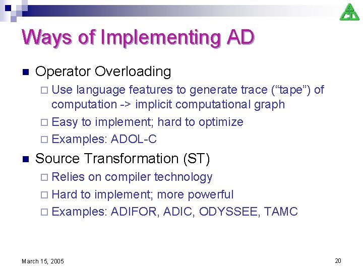
Ways of Implementing AD n Operator Overloading ¨ Use language features to generate trace (“tape”) of computation -> implicit computational graph ¨ Easy to implement; hard to optimize ¨ Examples: ADOL-C n Source Transformation (ST) ¨ Relies on compiler technology ¨ Hard to implement; more powerful ¨ Examples: ADIFOR, ADIC, ODYSSEE, TAMC March 15, 2005 20

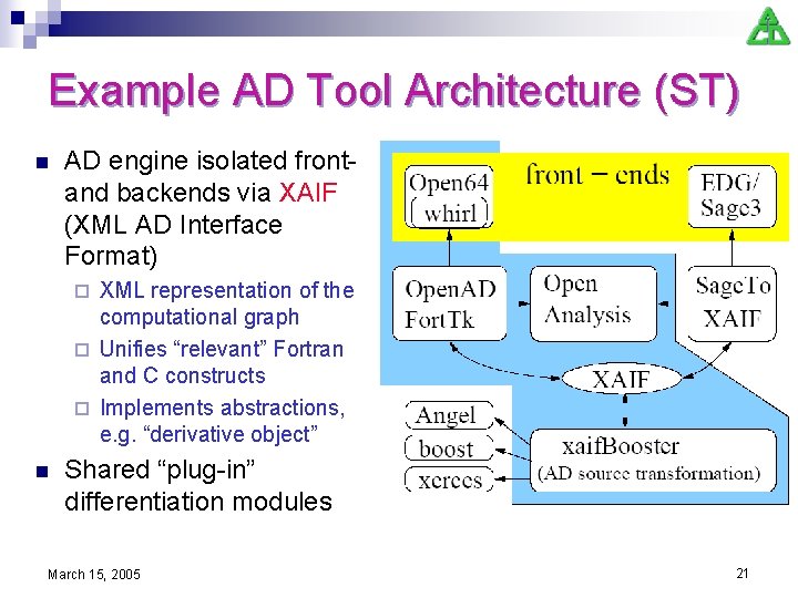
Example AD Tool Architecture (ST) n AD engine isolated frontand backends via XAIF (XML AD Interface Format) XML representation of the computational graph ¨ Unifies “relevant” Fortran and C constructs ¨ Implements abstractions, e. g. “derivative object” ¨ n Shared “plug-in” differentiation modules March 15, 2005 21

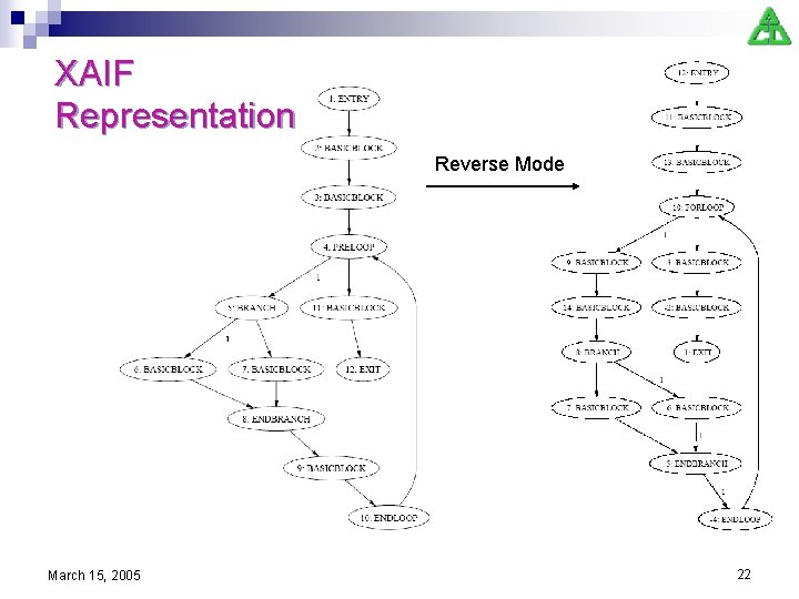
XAIF Representation Reverse Mode March 15, 2005 22

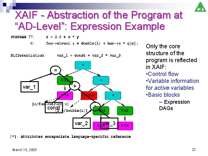
XAIF - Abstraction of the Program at “AD-Level”: Expression Example Only the core structure of the program is reflected in XAIF: • Control flow • Variable information for active variables • Basic blocks – Expression = + var_1 * const var_2 March 15, 2005 DAGs var_3 23

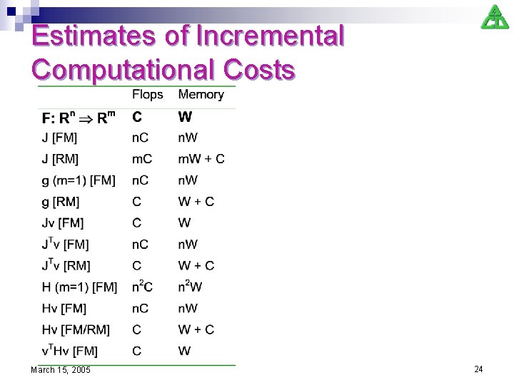
Estimates of Incremental Computational Costs March 15, 2005 24

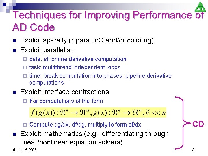
Techniques for Improving Performance of AD Code n n Exploit sparsity (Spars. Lin. C and/or coloring) Exploit parallelism data: stripmine derivative computation ¨ task: multithread independent loops ¨ time: break computation into phases; pipeline derivative computations ¨ n n Exploit interface contractions ¨ For computations of the form ¨ Compute dg/dx, df/dg, multiply to form df/dx CD Exploit mathematics (e. g. , differentiating through linear/nonlinear equation solvers) March 15, 2005 26

ANL Tools for AD n n n ADIFOR was developed in collaboration with Rice University ¨ full support for Fortran 77 ¨ support for parallelism via MPI and PVM ¨ support for sparse Jacobians ADIC is the first & only compiler-based AD tool for ANSI C ¨ support for the complete ANSI standard ¨ will soon support a large subset of C++ ¨ www. mcs. anl. gov/adic, www. mcs. anl. gov/adicserver XAIF specification and differentiation modules (Open. AD project) ¨ http: //www-unix. mcs. anl. gov/~utke/Open. AD March 15, 2005 27

AD in Numerical Toolkits n NEOS Network-Enabled Optimization Server ¨ http: //neos. mcs. anl. gov ¨ Efficient computation of gradients for large problems, where the objective function has the form n PETSc (Portable Extensible Toolkit for Scientific Computation) solvers (work in progress) ¨ User only needs to provide the sequential “subdomain update” function in F 77 or ANSI-C. ¨ Differentiated version of toolkit enables optimization/sensitivity analysis of models based on PETSc ¨ www. mcs. anl. gov/petsc 28 March 15, 2005

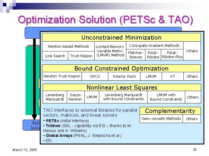
Optimization Solution (PETSc & TAO) Main Routine Unconstrained Minimization Newton-based Methods Line Search Limited Memory Variable Metric (LMVM) Method Trust Region Conjugate Gradient Methods Polak. Ribiére-Plus Fletcher. Reeves Others Nonlinear Solvers (SNES) Bound Constrained Optimization Newton Trust Region GPCG Interior Point LMVM Solve min F(u) Linear Solvers (SLES) KT Others Nonlinear Least Squares Levenberg Marquardt PC Gauss. Newton KSP LMVM Levenberg Marquardt with Bound Constraints LMVM with Others Numerical Bound Constraints Library Complementarity TAO interfaces to external libraries for parallel vectors, matrices, and linear solvers: Semi-smooth Methods Others • PETSc (initial interface) Application Minimum Function Gradient Hessian Post • Trilinos (SNL - capability via ESI – thanks to M. Initialization Evaluation Processing Heroux and A. Williams) • Global Arrays (PNNL, J. Nieplocha et al. ) • Etc. User code PETSc code AD-generated code March 15, 2005 29

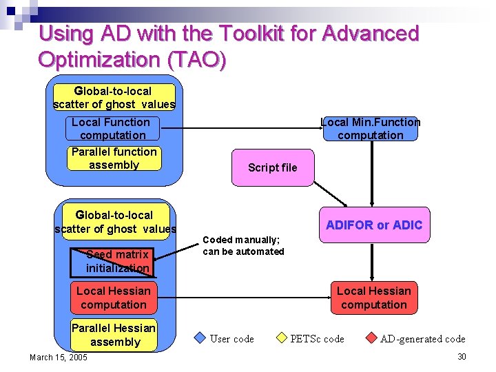
Using AD with the Toolkit for Advanced Optimization (TAO) Global-to-local scatter of ghost values Local Function computation Parallel function assembly Local Min. Function computation Script file Global-to-local scatter of ghost values Seed matrix initialization ADIFOR or ADIC Coded manually; can be automated Local Hessian computation Parallel Hessian assembly March 15, 2005 Local Hessian computation User code PETSc code AD-generated code 30

Outline n n Automatic differentiation Components for scientific computing ¨ Introduction ¨ Example n n applications Performance evaluation and modeling Summary CCA Common Component Architecture March 15, 2005 31

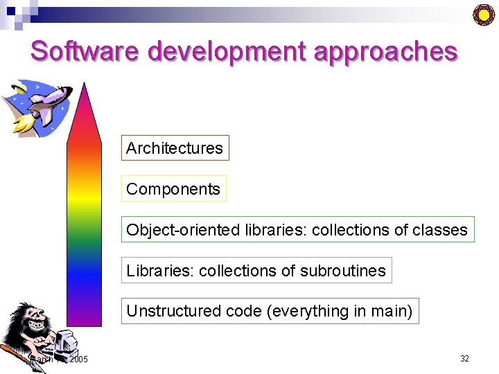
Software development approaches Architectures Components Object-oriented libraries: collections of classes Libraries: collections of subroutines Unstructured code (everything in main) March 15, 2005 32

Components n Working definition: a component is a piece of software that can be composed with other components within a framework; composition can be either static (at link time) or dynamic (at run time) “plug-and-play” model for building applications ¨ For more info: C. Szyperski, Component Software: Beyond Object. Oriented Programming, ACM Press, New York, 1998 ¨ n Components enable Software and tool interoperability ¨ Automation of performance instrumentation/monitoring ¨ Application adaptivity (automated or user-guided) ¨ n Pictorial intro March 15, 2005 33

Object-oriented vs component-oriented development n n n Component-oriented development can be viewed as augmenting OOD with certain policies, e. g. , require that certain abstract interfaces be implemented Components, once compiled, require a special execution environment OO techniques are useful for building individual components by relatively small teams; component technologies facilitate sharing of code developed by different groups by addressing issues in ¨ Language interoperability n ¨ Well-defined abstract interfaces n ¨ Enable “plug-and-play” Dynamic composability n n Via interface definition language (IDL) Components can discover information about their environment (e. g. , interface discovery) from framework and connected components Can convert from an object orientation to a component orientation ¨ Automatic tools can help with conversion (ongoing work by C. Rasmussen and M. Sottile, LANL) March 15, 2005 34

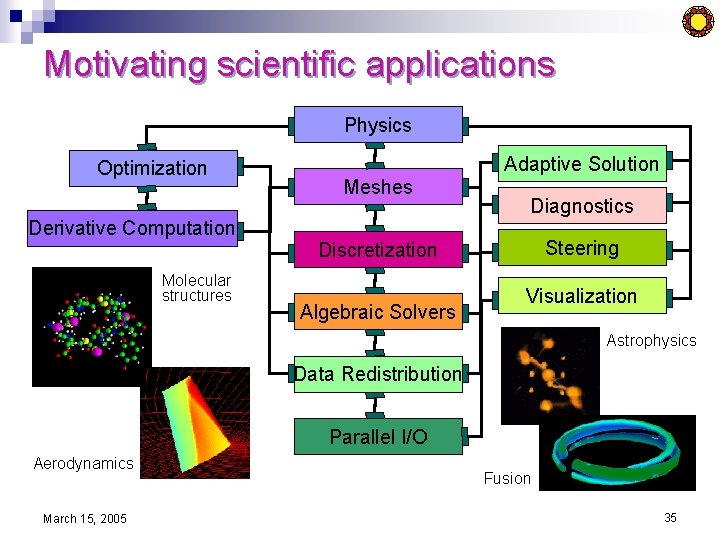
Motivating scientific applications Physics Optimization Derivative Computation Molecular structures Adaptive Solution Meshes Diagnostics Steering Discretization Algebraic Solvers Visualization Astrophysics Data Redistribution Parallel I/O Aerodynamics March 15, 2005 Fusion 35

Motivation: For Application Developers and Users n You have difficulty managing multiple third-party libraries in your code n You (want to) use more than two languages in your application n Your code is long-lived and different pieces evolve at different rates n You want to be able to swap competing implementations of the same idea and test without modifying any of your code n You want to compose your application with some other(s) that weren’t originally designed to be combined March 15, 2005 36

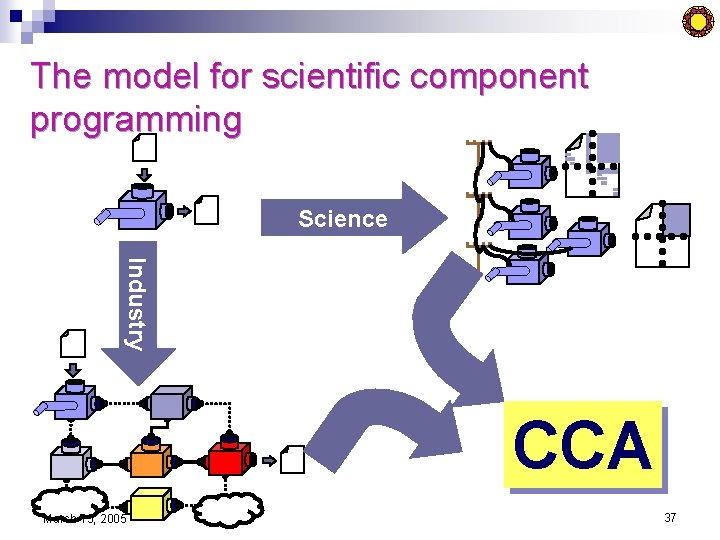
The model for scientific component programming Science Industry ? CA C March 15, 2005 37

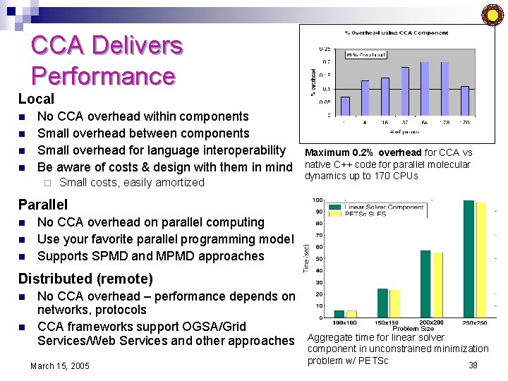
CCA Delivers Performance Local n n No CCA overhead within components Small overhead between components Small overhead for language interoperability Be aware of costs & design with them in mind ¨ Small costs, easily amortized Maximum 0. 2% overhead for CCA vs native C++ code for parallel molecular dynamics up to 170 CPUs Parallel n n n No CCA overhead on parallel computing Use your favorite parallel programming model Supports SPMD and MPMD approaches Distributed (remote) n n No CCA overhead – performance depends on networks, protocols CCA frameworks support OGSA/Grid Services/Web Services and other approaches March 15, 2005 Aggregate time for linear solver component in unconstrained minimization problem w/ PETSc 38

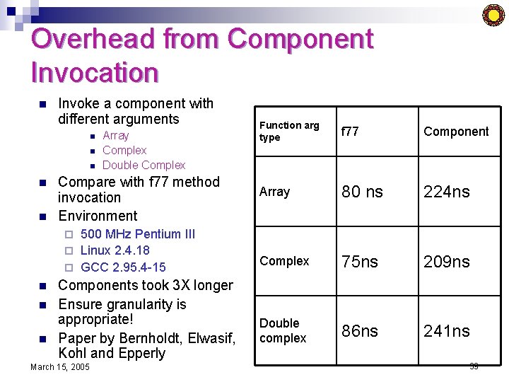
Overhead from Component Invocation n Invoke a component with different arguments n n n Array Complex Double Complex Compare with f 77 method invocation Environment 500 MHz Pentium III ¨ Linux 2. 4. 18 ¨ GCC 2. 95. 4 -15 Function arg type f 77 Component Array 80 ns 224 ns Complex 75 ns 209 ns Double complex 86 ns 241 ns ¨ n n n Components took 3 X longer Ensure granularity is appropriate! Paper by Bernholdt, Elwasif, Kohl and Epperly March 15, 2005 39

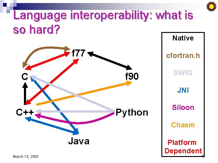
Language interoperability: what is so hard? Native f 77 cfortran. h f 90 C SWIG JNI C++ Python Siloon Chasm Java March 15, 2005 Platform Dependent 40

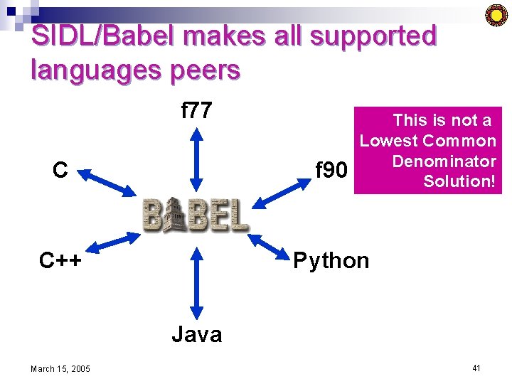
SIDL/Babel makes all supported languages peers f 77 This is not a Lowest Common Denominator Solution! C f 90 C++ Python Java March 15, 2005 41

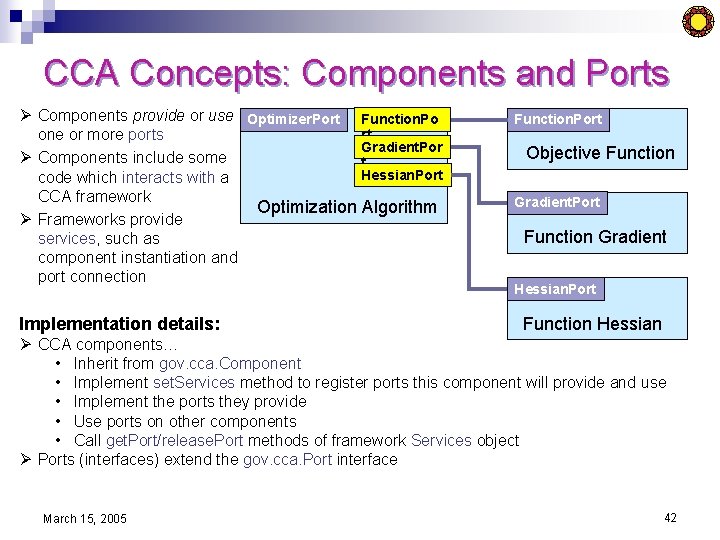
CCA Concepts: Components and Ports Ø Components provide or use Optimizer. Port Function. Po rt one or more ports Gradient. Por Ø Components include some t Hessian. Port code which interacts with a CCA framework Optimization Algorithm Ø Frameworks provide services, such as component instantiation and port connection Implementation details: Function. Port Objective Function Gradient. Port Function Gradient Hessian. Port Function Hessian Ø CCA components… • Inherit from gov. cca. Component • Implement set. Services method to register ports this component will provide and use • Implement the ports they provide • Use ports on other components • Call get. Port/release. Port methods of framework Services object Ø Ports (interfaces) extend the gov. cca. Port interface March 15, 2005 42

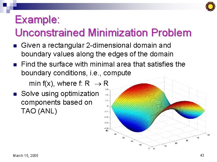
Example: Unconstrained Minimization Problem n n n Given a rectangular 2 -dimensional domain and boundary values along the edges of the domain Find the surface with minimal area that satisfies the boundary conditions, i. e. , compute min f(x), where f: R R Solve using optimization components based on TAO (ANL) March 15, 2005 43

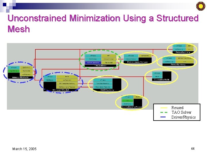
Unconstrained Minimization Using a Structured Mesh Reused TAO Solver Driver/Physics March 15, 2005 44

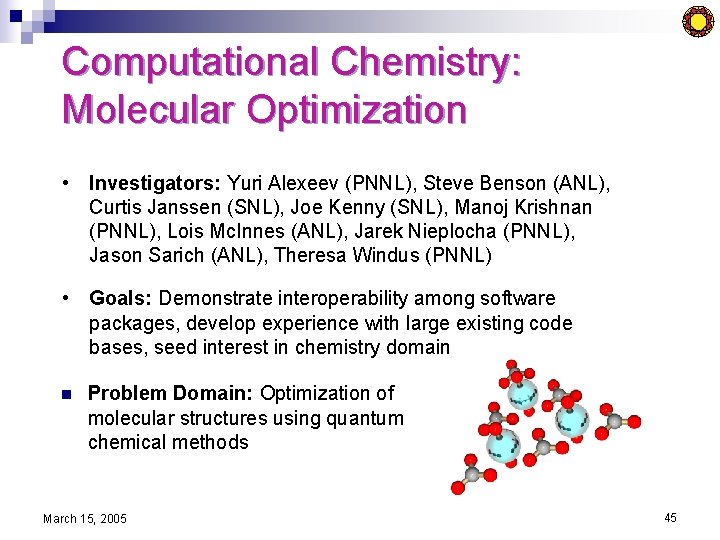
Computational Chemistry: Molecular Optimization • Investigators: Yuri Alexeev (PNNL), Steve Benson (ANL), Curtis Janssen (SNL), Joe Kenny (SNL), Manoj Krishnan (PNNL), Lois Mc. Innes (ANL), Jarek Nieplocha (PNNL), Jason Sarich (ANL), Theresa Windus (PNNL) • Goals: Demonstrate interoperability among software packages, develop experience with large existing code bases, seed interest in chemistry domain n Problem Domain: Optimization of molecular structures using quantum chemical methods March 15, 2005 45

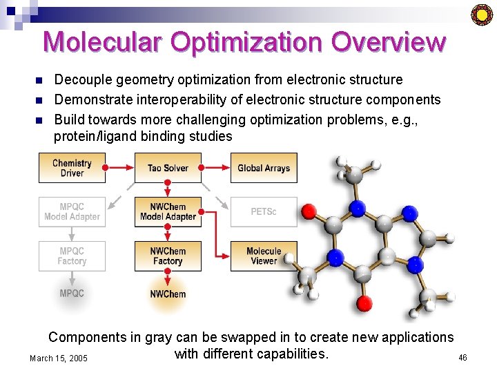
Molecular Optimization Overview n n n Decouple geometry optimization from electronic structure Demonstrate interoperability of electronic structure components Build towards more challenging optimization problems, e. g. , protein/ligand binding studies Components in gray can be swapped in to create new applications with different capabilities. 46 March 15, 2005

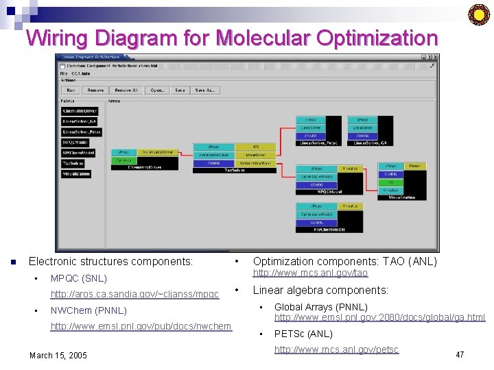
Wiring Diagram for Molecular Optimization n Electronic structures components: • Optimization components: TAO (ANL) • Linear algebra components: MPQC (SNL) http: //aros. ca. sandia. gov/~cljanss/mpqc • • NWChem (PNNL) http: //www. emsl. pnl. gov/pub/docs/nwchem March 15, 2005 http: //www. mcs. anl. gov/tao • Global Arrays (PNNL) http: //www. emsl. pnl. gov: 2080/docs/global/ga. html • PETSc (ANL) http: //www. mcs. anl. gov/petsc 47

Outline n n n Automatic differentiation Components for scientific computing Performance evaluation and modeling ¨ Performance evaluation challenges ¨ Component-based approach ¨ Motivating example: adaptive linear system solution ¨ A component infrastructure for performance monitoring and adaptation of applications n Summary March 15, 2005 48

Why Performance Model? n Performance models enable understanding of the factors that affect performance ¨ Inform the tuning process (of application and machine) n n Identify bottlenecks Identify underperforming components Guide applications to the best machine ¨ Enable applications-driven architecture design ¨ Extrapolate the performance of future systems ¨ March 15, 2005 49

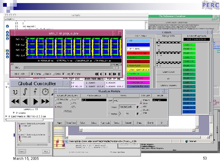
Challenges in performance evaluation + Many tools for performance data gathering and analysis ¨ ¨ PAPI, TAU, Sv. Pablo, Kojak, … Various interfaces, levels of automation, and approaches to information presentation Ø User’s point of view - What do the different tools do? Which is most appropriate for a given application? - (How) can multiple tools be used in concert? - I have tons of performance data, now what? - What automatic tuning tools are available, what exactly do they do? - How hard is it to install/learn/use tool X? - Is instrumented code portable? What’s the overhead of instrumentation? How does code evolution affect the performance analysis process? March 15, 2005 50

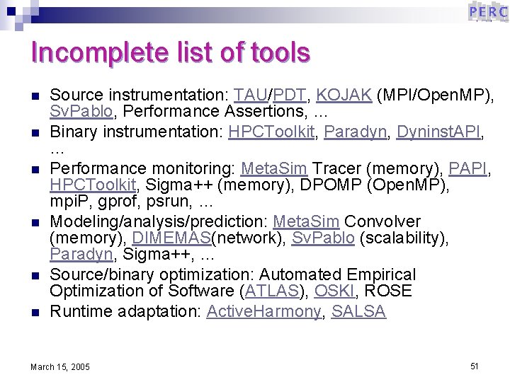
Incomplete list of tools n n n Source instrumentation: TAU/PDT, KOJAK (MPI/Open. MP), Sv. Pablo, Performance Assertions, … Binary instrumentation: HPCToolkit, Paradyn, Dyninst. API, … Performance monitoring: Meta. Sim Tracer (memory), PAPI, HPCToolkit, Sigma++ (memory), DPOMP (Open. MP), mpi. P, gprof, psrun, … Modeling/analysis/prediction: Meta. Sim Convolver (memory), DIMEMAS(network), Sv. Pablo (scalability), Paradyn, Sigma++, … Source/binary optimization: Automated Empirical Optimization of Software (ATLAS), OSKI, ROSE Runtime adaptation: Active. Harmony, SALSA March 15, 2005 51

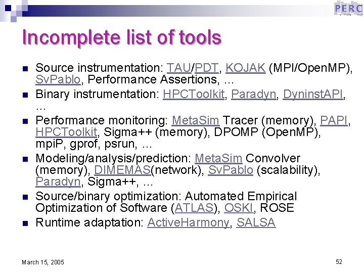
Incomplete list of tools n n n Source instrumentation: TAU/PDT, KOJAK (MPI/Open. MP), Sv. Pablo, Performance Assertions, … Binary instrumentation: HPCToolkit, Paradyn, Dyninst. API, … Performance monitoring: Meta. Sim Tracer (memory), PAPI, HPCToolkit, Sigma++ (memory), DPOMP (Open. MP), mpi. P, gprof, psrun, … Modeling/analysis/prediction: Meta. Sim Convolver (memory), DIMEMAS(network), Sv. Pablo (scalability), Paradyn, Sigma++, … Source/binary optimization: Automated Empirical Optimization of Software (ATLAS), OSKI, ROSE Runtime adaptation: Active. Harmony, SALSA March 15, 2005 52

Incomplete list of tools n n n Source instrumentation: TAU/PDT, KOJAK (MPI/Open. MP), Sv. Pablo, Performance Assertions, … Binary instrumentation: HPCToolkit, Paradyn, Dyninst. API, … Performance monitoring: Meta. Sim Tracer (memory), PAPI, HPCToolkit, Sigma++ (memory), DPOMP (Open. MP), mpi. P, gprof, psrun, … Modeling/analysis/prediction: Meta. Sim Convolver (memory), DIMEMAS(network), Sv. Pablo (scalability), Paradyn, Sigma++, … Source/binary optimization: Automated Empirical Optimization of Software (ATLAS), OSKI, ROSE Runtime adaptation: Active. Harmony, SALSA March 15, 2005 53

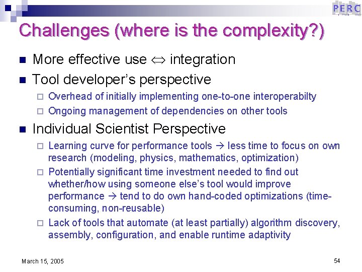
Challenges (where is the complexity? ) n n More effective use integration Tool developer’s perspective Overhead of initially implementing one-to-one interoperabilty ¨ Ongoing management of dependencies on other tools ¨ n Individual Scientist Perspective Learning curve for performance tools less time to focus on own research (modeling, physics, mathematics, optimization) ¨ Potentially significant time investment needed to find out whether/how using someone else’s tool would improve performance tend to do own hand-coded optimizations (timeconsuming, non-reusable) ¨ Lack of tools that automate (at least partially) algorithm discovery, assembly, configuration, and enable runtime adaptivity ¨ March 15, 2005 54

What can be done n How to manage complexity? Provide ¨ Performance tools that are truly interoperable ¨ Uniform easy access to tools ¨ Component implementations of software, esp. supporting numerical codes, such as linear algebra algorithms ¨ New algorithms (e. g. , interactive/dynamic techniques, algorithm composition) n Implementation approach: components, both for tools and the application software March 15, 2005 55

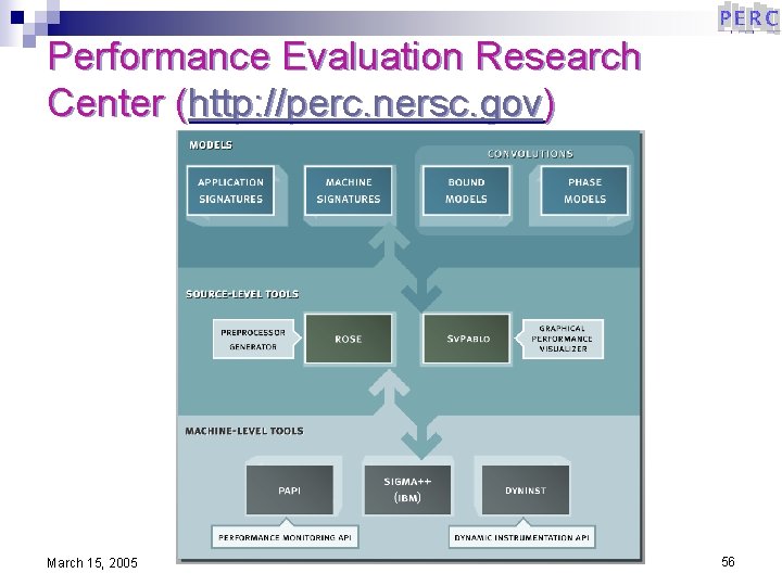
Performance Evaluation Research Center (http: //perc. nersc. gov) March 15, 2005 56

What is being done n n No “integrated” environment for performance monitoring, analysis, and optimization (yet) Most past efforts ¨ One-to-one n tool interoperability More recently ¨ OSPAT (initial meeting at SC’ 04), focus on common data representation and interfaces ¨ Tool-independent performance databases: Perf. DMF ¨ Eclipse parallel tools project (LANL) ¨… March 15, 2005 57

Example: component infrastructure for multimethod linear solvers n Goal: provide a framework for Performance monitoring of numerical components ¨ Dynamic adaptativity, based on: ¨ n n n Off-line analyses of past performance information Online analysis of current execution performance information Motivating application examples: Driven cavity flow [Coffey et al, 2003], nonlinear PDE solution ¨ FUN 3 D – incompressible and compressible Euler equations ¨ n Prior work in multimethod linear solvers ¨ Mc. Innes et al, ’ 03, Bhowmick et al, ’ 03 and ’ 05, Norris at al. ’ 05. March 15, 2005 59

Adaptive Linear System Solution n Motivation: Approximately 80% of total solution time devoted to linear system solution ¨ Multi-phase nonlinear solution method, requiring the solution of linear systems with varying levels of ill-conditioning [Kelley and Keyes, 1998] ¨ n New approach aiming to reduce overall time to solution Combine more robust (but more costly) methods when needed in some phases with faster (but less powerful) methods in other phases ¨ Dynamically select a new preconditioner in each phase based on CFL number ¨ March 15, 2005 60

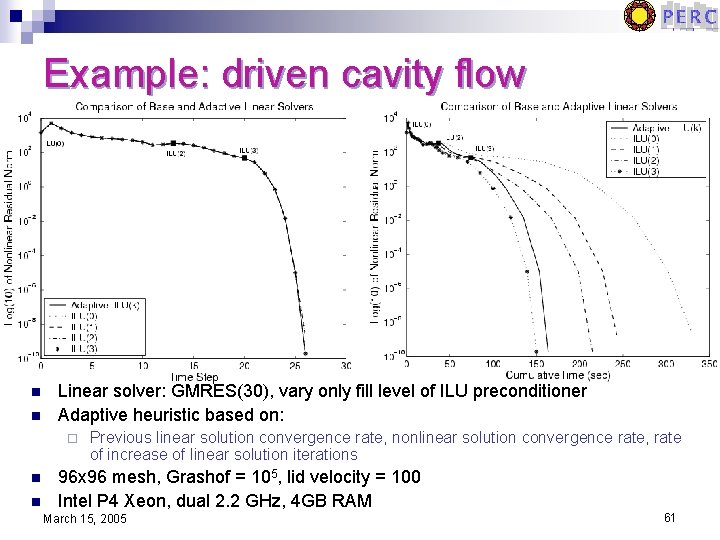
Example: driven cavity flow n n Linear solver: GMRES(30), vary only fill level of ILU preconditioner Adaptive heuristic based on: ¨ n n Previous linear solution convergence rate, nonlinear solution convergence rate, rate of increase of linear solution iterations 96 x 96 mesh, Grashof = 105, lid velocity = 100 Intel P 4 Xeon, dual 2. 2 GHz, 4 GB RAM March 15, 2005 61

Bringing it all together n Integration of ongoing efforts in ¨ Performance tools: common interfaces and data represenation (leverage OSPAT, Perf. DMF, TAU performance interfaces, and similar efforts) ¨ Numerical components: emerging common interfaces (e. g. , TOPS solver interfaces) increase choice of solution method automated composition and adaptation strategies ¨ Code generation, e. g. , AD n Long term ¨ Is a more organized (but not too restrictive) environment for scientific software lifecycle development possible/desirable? March 15, 2005 62

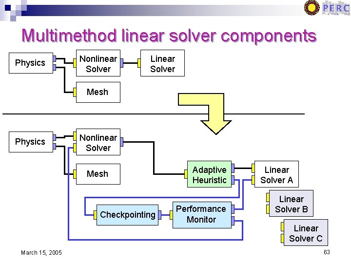
Multimethod linear solver components Physics Nonlinear Solver Linear Solver Mesh Physics Nonlinear Solver Mesh Checkpointing March 15, 2005 Adaptive Heuristic Performance Monitor Linear Solver A Linear Solver B Linear Solver C 63

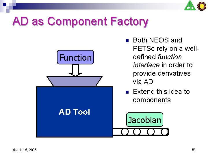
AD as Component Factory n Function n AD Tool March 15, 2005 Both NEOS and PETSc rely on a welldefined function interface in order to provide derivatives via AD Extend this idea to components Jacobian 64

Summary n Automation at all levels of the application development process can simplify and speed up application development and result in better software quality and performance AD addresses the wide-spread need for accurate and efficient derivative computations ¨ CCA defines a high-performance component model, enabling large-scale software development ¨ A growing array of performance tools and methodologies aid in understanding and fine-tuning application performance ¨ n Current and future work: bringing these technologies together in a coherent way, making large-scale scientific application development as easy as possible March 15, 2005 65

Acknowledgments n n n Paul Hovland, Jean Utke, Lois Curfman Mc. Innes (ANL) Sanjukta Bhowmick (ANL/Columbia) Ivana Veljkovic, Padma Raghavan (Penn State) Sameer Shende, Al Malony (U. Oregon) CCA and PERC members Funding: DOE and NSF March 15, 2005 66

For More Information n Automatic differentiation ¨ Andreas Griewank. Evaluating Derivatives: Principles and Techniques of Alogrithmic Differentiation, SIAM, 2000. www. autodiff. org : publications, tools, etc. ¨ www. mcs. anl. gov/adicserver : ADIC server ¨ neos. mcs. anl. gov : NEOS server ¨ n Common component architecture ¨ n Performance tools ¨ n perc. nersc. gov Student opportunities at MCS/ANL ¨ n www. cca-forum. org wwwfp. mcs. anl. gov/division/information/educational_programs/studento pps. html Boyana Norris March 15, 2005 67