Technoeconomic aspects of power systems Ronnie Belmans Dirk

Techno-economic aspects of power systems Ronnie Belmans Dirk Van Hertem Stijn Cole © K. U. Leuven - ESAT/Electa

Overview • • • Lesson 1: Liberalization Lesson 2: Players, Functions and Tasks Lesson 3: Markets Lesson 4: Present generation park Lesson 5: Future generation park Lesson 6: Introduction to power systems Lesson 7: Power system analysis and control Lesson 8: Power system dynamics and security Lesson 9: Future grid technologies: FACTS and HVDC Lesson 10: Distributed generation © K. U. Leuven - ESAT/Electa

Outline Power system analysis and control • Power system analysis Power flow § Optimal power flow § • Power flow control Primary control § Secondary control § Tertiary control § Voltage control § © K. U. Leuven - ESAT/Electa

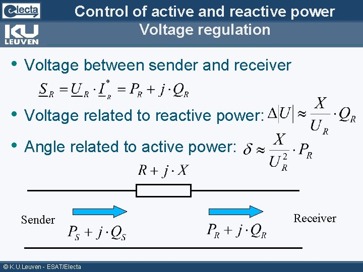
Control of active and reactive power Voltage regulation • Voltage between sender and receiver • Voltage related to reactive power: • Angle related to active power: Sender © K. U. Leuven - ESAT/Electa Receiver

Power flow • Normal conditions ==> steady state (equilibrium) • Basis calculations to obtain this state are called Power Flow § Also called Load Flow • Purpose of power flow: Determine steady state situation of the grid § Get values for P, Q, U and voltage angle § Calculate system losses § First step for § o o o N-1 contingency study Congestion analysis Need for redispatch System development Stability studies. . . © K. U. Leuven - ESAT/Electa

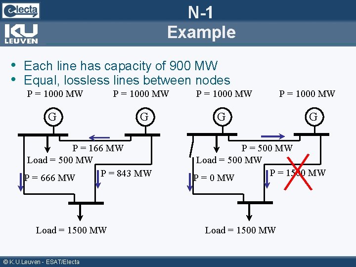
N-1 Example • Each line has capacity of 900 MW • Equal, lossless lines between nodes P = 1000 MW G P = 166 MW Load = 500 MW P = 843 MW P = 666 MW Load = 1500 MW © K. U. Leuven - ESAT/Electa P = 1000 MW G P = 500 MW Load = 500 MW P = 1500 MW P = 0 MW Load = 1500 MW

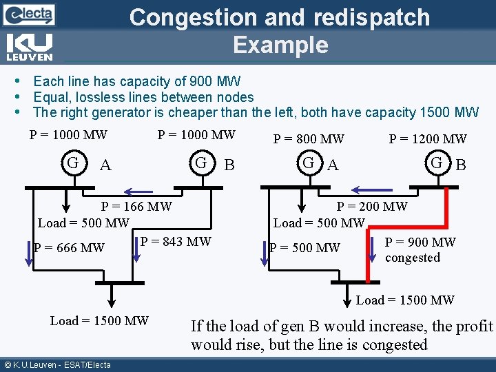
Congestion and redispatch Example • Each line has capacity of 900 MW • Equal, lossless lines between nodes • The right generator is cheaper than the left, both have capacity 1500 MW P = 1000 MW G G A P = 166 MW Load = 500 MW P = 843 MW P = 666 MW B P = 800 MW G A P = 1200 MW G B P = 200 MW Load = 500 MW P = 900 MW P = 500 MW congested Load = 1500 MW © K. U. Leuven - ESAT/Electa If the load of gen B would increase, the profit would rise, but the line is congested

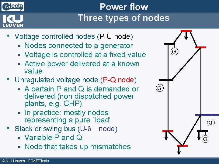
Power flow Three types of nodes • Voltage controlled nodes (P-U node) Nodes connected to a generator Voltage is controlled at a fixed value Active power delivered at a known value • Unregulated voltage node (P-Q node) § A certain P and Q is demanded or delivered (non dispatched power plants, e. g. CHP) § In practice: mostly nodes representing a pure `load' • Slack or swing bus (U- node) § Variable P and Q § Node that takes up mismatches § § § © K. U. Leuven - ESAT/Electa G G

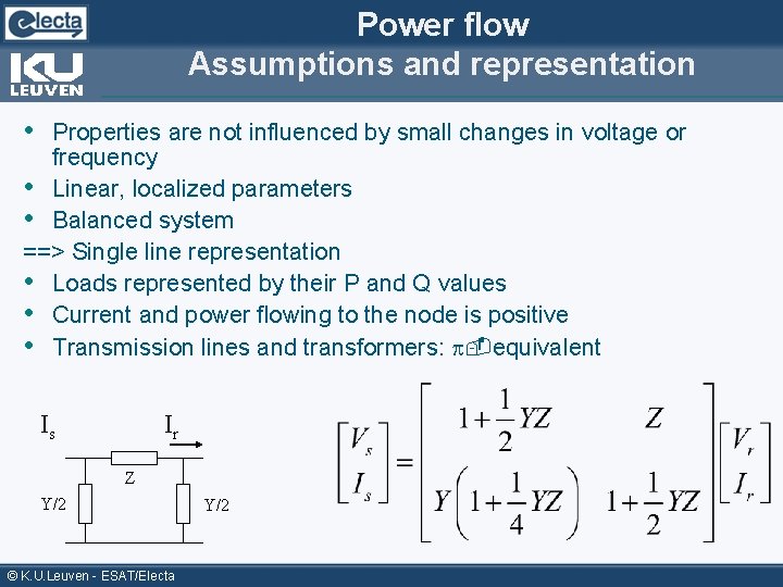
Power flow Assumptions and representation • Properties are not influenced by small changes in voltage or frequency • Linear, localized parameters • Balanced system ==> Single line representation • Loads represented by their P and Q values • Current and power flowing to the node is positive • Transmission lines and transformers: -equivalent Is Ir Z Y/2 © K. U. Leuven - ESAT/Electa Y/2

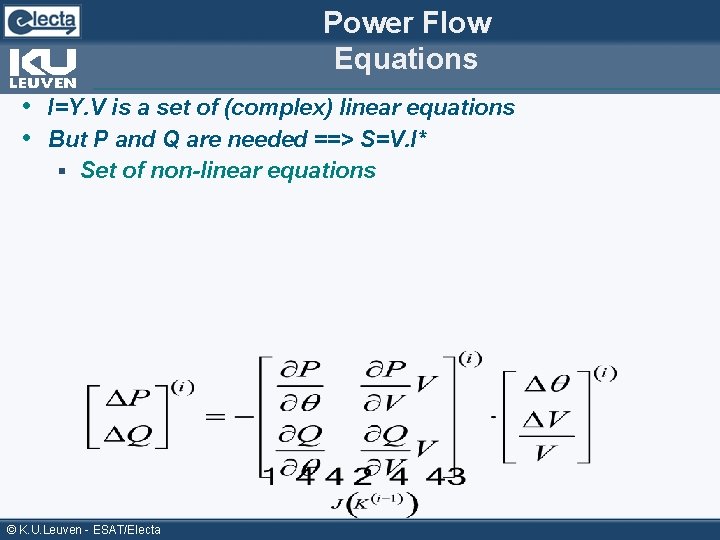
Power Flow Equations • I=Y. V is a set of (complex) linear equations • But P and Q are needed ==> S=V. I* § Set of non-linear equations © K. U. Leuven - ESAT/Electa

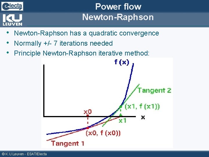
Power flow Newton-Raphson • Newton-Raphson has a quadratic convergence • Normally +/- 7 iterations needed • Principle Newton-Raphson iterative method: © K. U. Leuven - ESAT/Electa

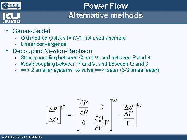
Power Flow Alternative methods • Gauss-Seidel § § Old method (solves I=Y. V), not used anymore Linear convergence § § § Strong coupling between Q and V, and between P and Weak coupling between P and V, and between Q and ==> 2 smaller systems to solve ==> faster (2 -3 times faster) • Decoupled Newton-Raphson © K. U. Leuven - ESAT/Electa

Power Flow Alternative methods (II) • Fast decoupled Newton-Raphson Neglects coupling as in decoupled Newton-Raphson § Approximation: Jacobian considered constant § • Newton-Raphson with convergence parameter § Step in right direction (first order) multiplied by factor • DC load flow § § § Consider only B (not Y) Single calculation (no iterations needed) Very fast ==> 7 -10 times faster than normal Newton-Raphson In high voltage grids: 1 pu Sometimes used as first value for Newton-Raphson iteration (starting value) Economic studies and contingency analysis also use DC load flow © K. U. Leuven - ESAT/Electa

Power flow: Available computer tools • Available programs: § § § § PSS/E (Siemens) Dig. SILENT ETAP Powerworld (demo version available for download) Matpower (free download, matlab based) PSAT: power system analysis toolbox (free download, matlab based). . . © K. U. Leuven - ESAT/Electa

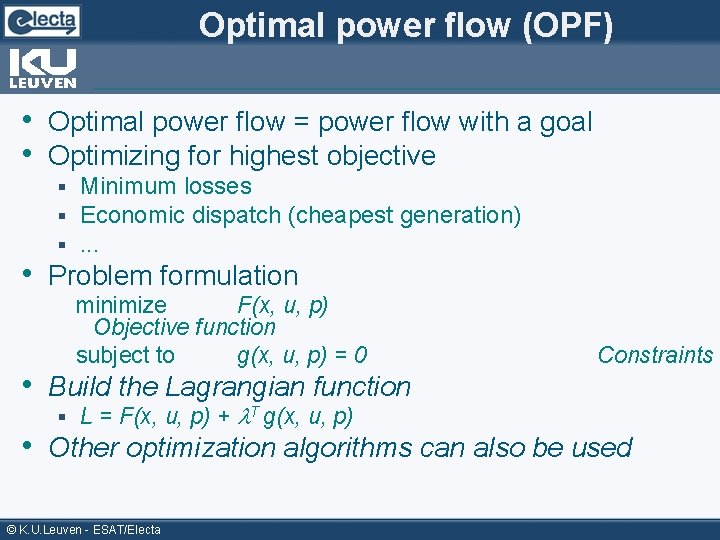
Optimal power flow (OPF) • Optimal power flow = power flow with a goal • Optimizing for highest objective § § § Minimum losses Economic dispatch (cheapest generation). . . • Problem formulation minimize F(x, u, p) Objective function subject to g(x, u, p) = 0 • Build the Lagrangian function § L = F(x, u, p) + T g(x, u, p) Constraints • Other optimization algorithms can also be used © K. U. Leuven - ESAT/Electa

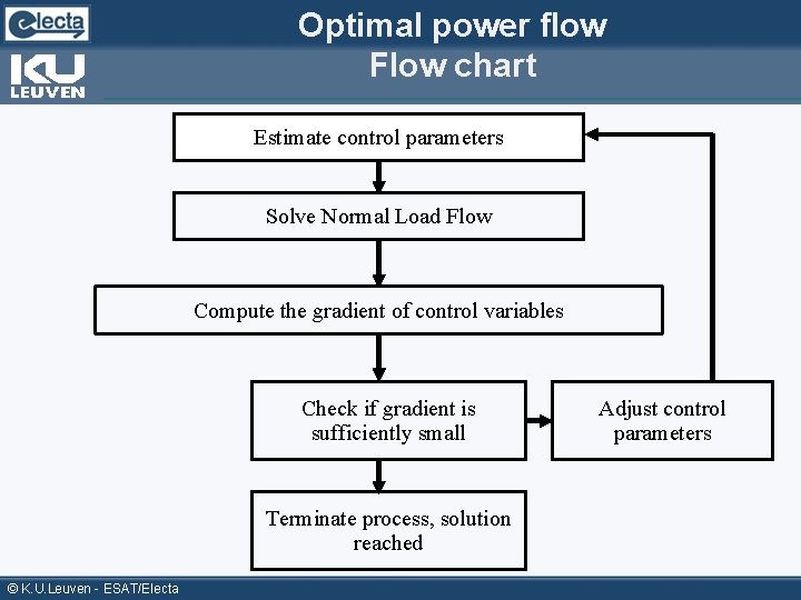
Optimal power flow Flow chart Estimate control parameters Solve Normal Load Flow Compute the gradient of control variables Check if gradient is sufficiently small Terminate process, solution reached © K. U. Leuven - ESAT/Electa Adjust control parameters

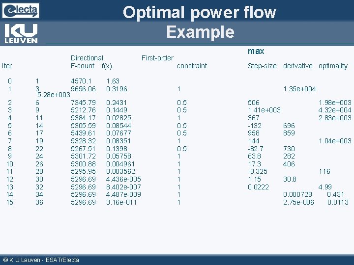
Optimal power flow Example Iter 0 1 2 3 4 5 6 7 8 9 10 11 12 13 14 15 Directional F-count f(x) 1 4570. 1 3 9656. 06 5. 28 e+003 6 7345. 79 9 5212. 76 11 5384. 17 14 5305. 59 17 5439. 61 19 5328. 32 22 5267. 51 24 5301. 72 26 5300. 88 28 5295. 95 30 5296. 69 32 5296. 69 34 5296. 69 36 5296. 69 © K. U. Leuven - ESAT/Electa max First-order constraint 1. 63 0. 3196 1 0. 2431 0. 1449 0. 02825 0. 08544 0. 07677 0. 08351 0. 1398 0. 05758 0. 004961 0. 003562 4. 436 e-005 8. 402 e-007 4. 487 e-009 3. 16 e-011 0. 5 1 0. 5 1 1 1 1 Step-size derivative optimality 1. 35 e+004 506 1. 41 e+003 367 -132 958 144 -82. 7 63. 8 17. 3 -0. 325 1. 15 0. 0222 696 859 730 282 406 30. 8 1. 98 e+003 4. 32 e+004 2. 83 e+003 1. 04 e+003 116 4. 99 0. 000728 0. 431 2. 75 e-006 0. 0113

Outline Power system analysis and control • Power system analysis Power flow § Optimal power flow § • Power flow control Primary control § Secondary control § Tertiary control § Voltage control § © K. U. Leuven - ESAT/Electa

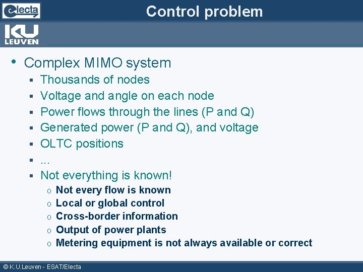
Control problem • Complex MIMO system § § § § Thousands of nodes Voltage and angle on each node Power flows through the lines (P and Q) Generated power (P and Q), and voltage OLTC positions. . . Not everything is known! o o o Not every flow is known Local or global control Cross-border information Output of power plants Metering equipment is not always available or correct © K. U. Leuven - ESAT/Electa

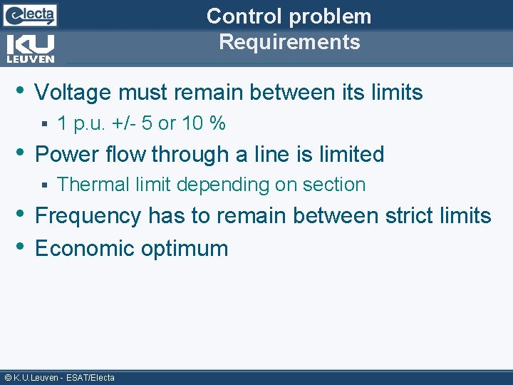
Control problem Requirements • Voltage must remain between its limits § 1 p. u. +/- 5 or 10 % • Power flow through a line is limited § Thermal limit depending on section • Frequency has to remain between strict limits • Economic optimum © K. U. Leuven - ESAT/Electa

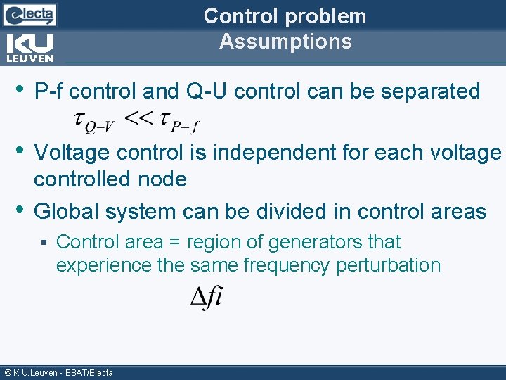
Control problem Assumptions • P-f control and Q-U control can be separated • Voltage control is independent for each voltage • controlled node Global system can be divided in control areas § Control area = region of generators that experience the same frequency perturbation © K. U. Leuven - ESAT/Electa

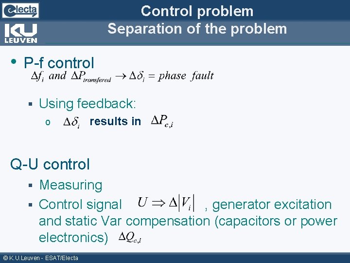
Control problem Separation of the problem • P-f control § Using feedback: o results in Q-U control Measuring § Control signal , generator excitation and static Var compensation (capacitors or power electronics) § © K. U. Leuven - ESAT/Electa

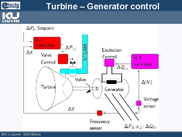
Turbine – Generator control © K. U. Leuven - ESAT/Electa

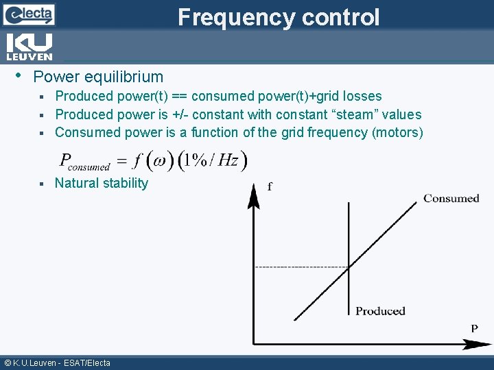
Frequency control • Power equilibrium Produced power(t) == consumed power(t)+grid losses § Produced power is +/- constant with constant “steam” values § Consumed power is a function of the grid frequency (motors) § § Natural stability © K. U. Leuven - ESAT/Electa

Why frequency control? • Uncontrolled power variations affect machine speed • Frequency has to remain between very strict limits © K. U. Leuven - ESAT/Electa

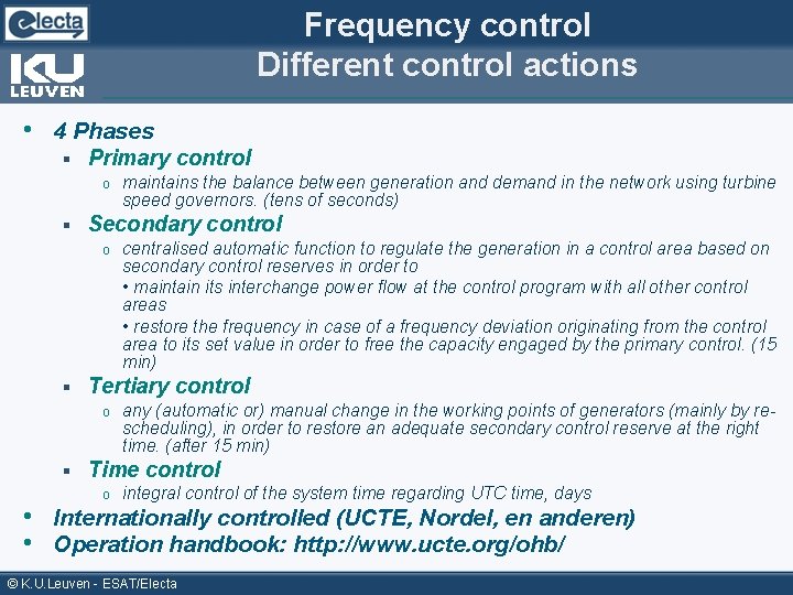
Frequency control Different control actions • 4 Phases § Primary control o § Secondary control o § centralised automatic function to regulate the generation in a control area based on secondary control reserves in order to • maintain its interchange power flow at the control program with all other control areas • restore the frequency in case of a frequency deviation originating from the control area to its set value in order to free the capacity engaged by the primary control. (15 min) Tertiary control o § maintains the balance between generation and demand in the network using turbine speed governors. (tens of seconds) any (automatic or) manual change in the working points of generators (mainly by rescheduling), in order to restore an adequate secondary control reserve at the right time. (after 15 min) Time control o integral control of the system time regarding UTC time, days • Internationally controlled (UCTE, Nordel, en anderen) • Operation handbook: http: //www. ucte. org/ohb/ © K. U. Leuven - ESAT/Electa

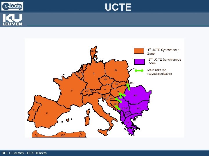
UCTE © K. U. Leuven - ESAT/Electa

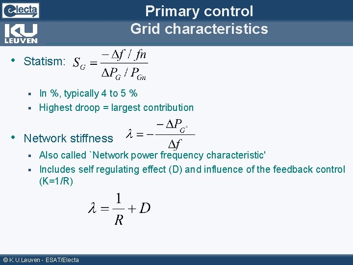
Primary control Grid characteristics • Statism: In %, typically 4 to 5 % § Highest droop = largest contribution § • Network stiffness Also called `Network power frequency characteristic' § Includes self regulating effect (D) and influence of the feedback control (K=1/R) § © K. U. Leuven - ESAT/Electa

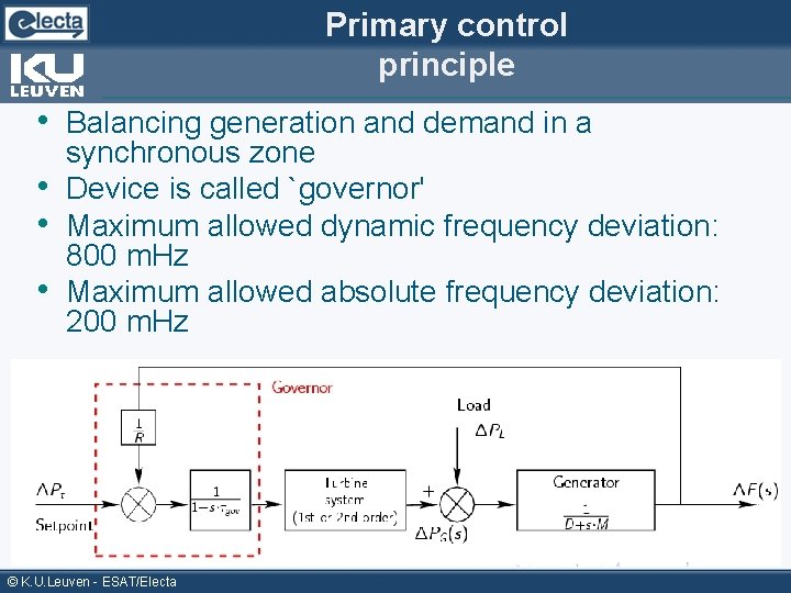
Primary control principle • Balancing generation and demand in a • • • synchronous zone Device is called `governor' Maximum allowed dynamic frequency deviation: 800 m. Hz Maximum allowed absolute frequency deviation: 200 m. Hz © K. U. Leuven - ESAT/Electa

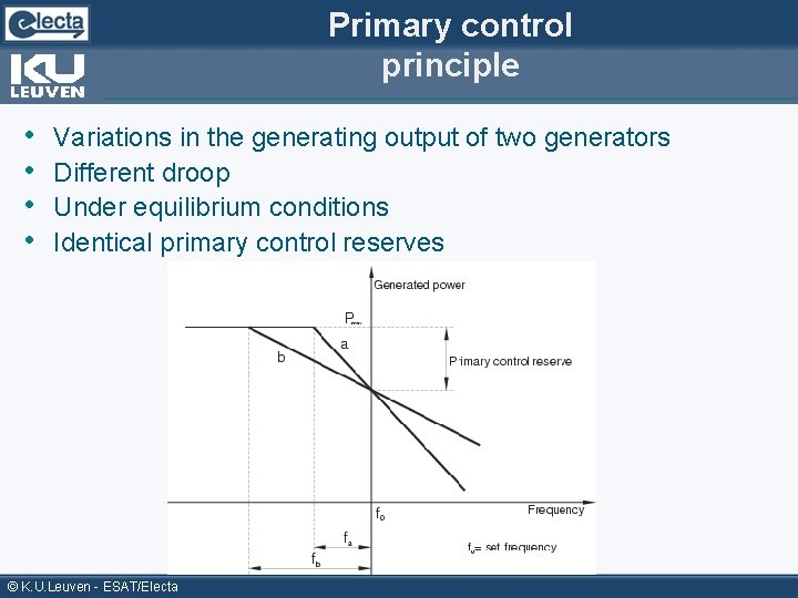
Primary control principle • • Variations in the generating output of two generators Different droop Under equilibrium conditions Identical primary control reserves © K. U. Leuven - ESAT/Electa

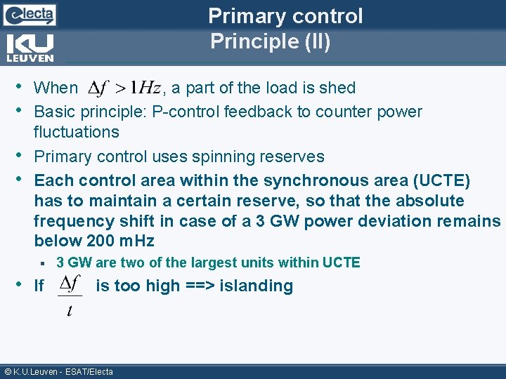
Primary control Principle (II) • When , a part of the load is shed • Basic principle: P-control feedback to counter power • • fluctuations Primary control uses spinning reserves Each control area within the synchronous area (UCTE) has to maintain a certain reserve, so that the absolute frequency shift in case of a 3 GW power deviation remains below 200 m. Hz § • If 3 GW are two of the largest units within UCTE is too high ==> islanding © K. U. Leuven - ESAT/Electa

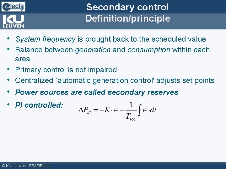
Secondary control Definition/principle • System frequency is brought back to the scheduled value • Balance between generation and consumption within each area Primary control is not impaired Centralized `automatic generation control' adjusts set points • • • Power sources are called secondary reserves • PI controlled: © K. U. Leuven - ESAT/Electa

Primary and secondary control Example © K. U. Leuven - ESAT/Electa

Primary and secondary control Example (II) © K. U. Leuven - ESAT/Electa

Primary and secondary control Example (III) © K. U. Leuven - ESAT/Electa

Primary and secondary control Example (IV) © K. U. Leuven - ESAT/Electa

Primary and secondary control Example (V) © K. U. Leuven - ESAT/Electa

Primary and secondary control Example (VI) This phase happens simultaneously with the secondary control, and the “ 50. 1 Hz” in reality doesn't occur © K. U. Leuven - ESAT/Electa

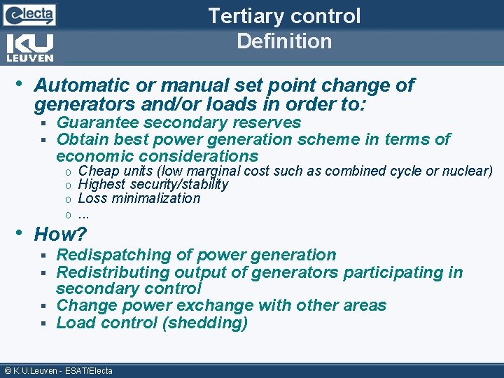
Tertiary control Definition • Automatic or manual set point change of generators and/or loads in order to: § § Guarantee secondary reserves Obtain best power generation scheme in terms of economic considerations o o Cheap units (low marginal cost such as combined cycle or nuclear) Highest security/stability Loss minimalization. . . • How? Redispatching of power generation Redistributing output of generators participating in secondary control § Change power exchange with other areas § Load control (shedding) § § © K. U. Leuven - ESAT/Electa

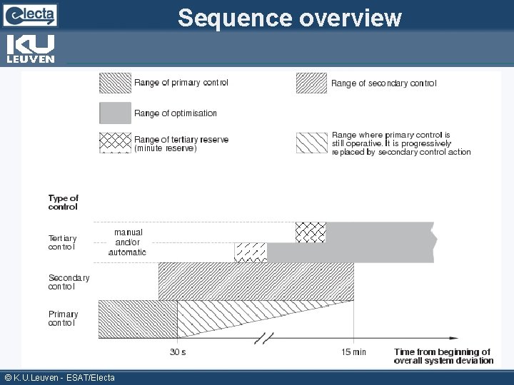
Sequence overview © K. U. Leuven - ESAT/Electa

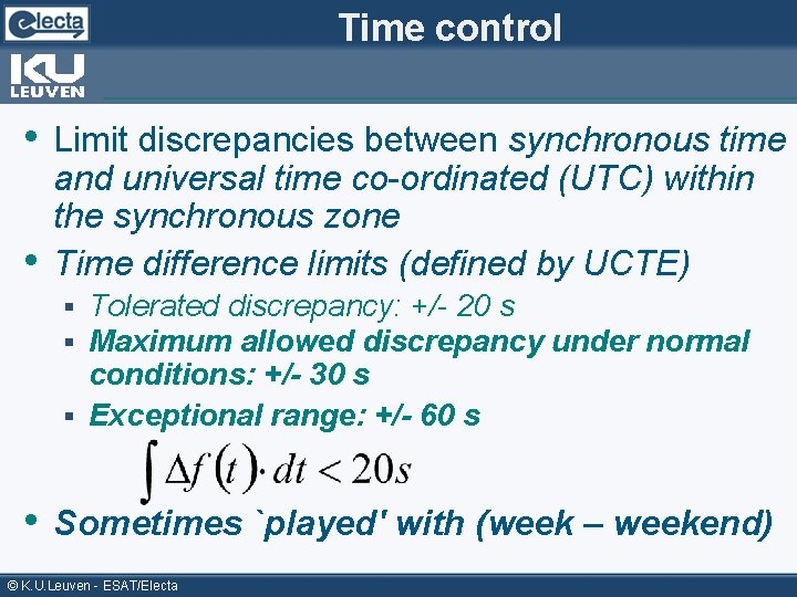
Time control • Limit discrepancies between synchronous time • and universal time co-ordinated (UTC) within the synchronous zone Time difference limits (defined by UCTE) Tolerated discrepancy: +/- 20 s Maximum allowed discrepancy under normal conditions: +/- 30 s § Exceptional range: +/- 60 s § § • Sometimes `played' with (week – weekend) © K. U. Leuven - ESAT/Electa

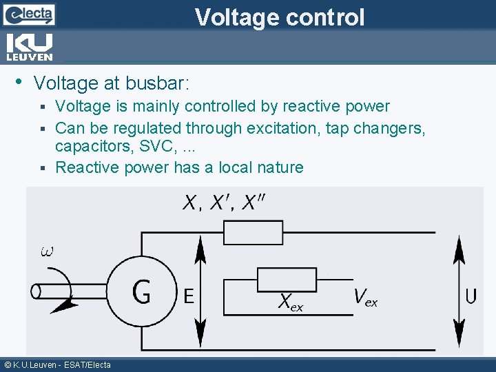
Voltage control • Voltage at busbar: Voltage is mainly controlled by reactive power § Can be regulated through excitation, tap changers, capacitors, SVC, . . . § Reactive power has a local nature § © K. U. Leuven - ESAT/Electa

Voltage control • Can the same control mechanism be used? § YES • But § Good (sensitive) Q-production has to be available Synchronous compensator: expensive o Capacitors: not accurate enough o SVC/STATCom: possible, but not cheap o U is `OK' between 0, 95 and 1, 05 p. u. § Reactive power is less price (fuel) dependent (some losses) § • Voltage is locally controlled © K. U. Leuven - ESAT/Electa

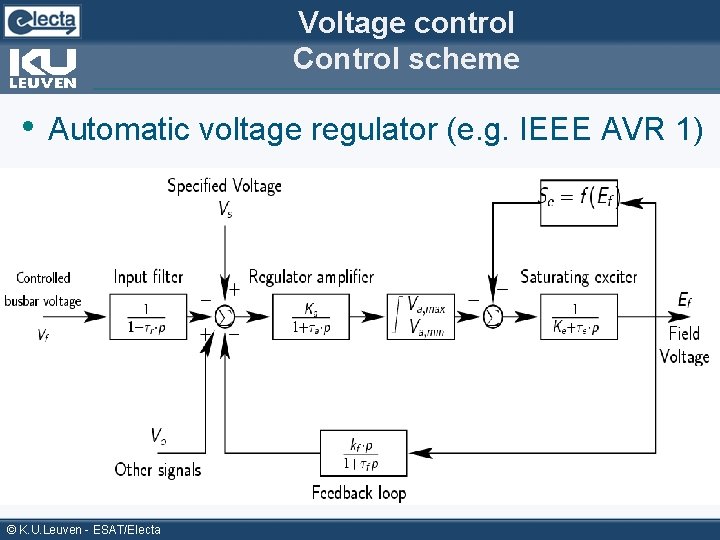
Voltage control Control scheme • Automatic voltage regulator (e. g. IEEE AVR 1) © K. U. Leuven - ESAT/Electa

Conclusions • Power flow analysis Performed through iterative method (Newton. Raphson) § Basis for many power system studies § Optimal power flow § • Power flow control happens in several independent stages Inter-area ties make the grid more reliable § Voltage control is independent of power (frequency) control § © K. U. Leuven - ESAT/Electa

References • Power System Stability and control, Prabha • • • Kundur, 1994, Mc. Graw-Hill Operational handbook UCTE, http: //www. ucte. org/ohb/cur_status. asp Power system dynamics: stability and control, K. Padiyar, Ansham, 2004 Power system analysis, Grainger and Stevenson Power system control and stability, 2 nd ed. , Andersson and Fouad Dynamics and Control of Electric Power Systems, Goran Andersson © K. U. Leuven - ESAT/Electa