Techniques Based on Recursion n How to design

Techniques Based on Recursion n How to design and solve recursion?

4. 1 Design recursion algorithm n n n Recursion (递归) is one of most powerful methods of solution available to computer scientists. Recursion is a problem-solving approach that can be used to generate simple solutions to certain kinds of problems that would be difficult to solve in other ways. Recursion splits (划分) a problem into one or more simpler versions of itself. 2

Steps to Design a Recursive Algorithm n n n There must be at least one case (the base case), for a small value of n, that can be solved directly. A problem of a given size n can be split into one or more smaller versions of the same problem (recursive case) Recognize the base case and provide a solution to it Devise a strategy to split the problem into smaller versions of itself while making progress toward the base case Combine the solutions of the smaller problems in such a way as to solve the larger problem 3

n These are questions to answer when using recursive solution: n n How can you define the problem in terms of a smaller problem of the same type? How does each recursive call diminish the size of the problem? What instance of the problem can serve as the base case? As the problem size diminishes, will you reach this base case? 4

So, why use recursion? n n Advantages. . . n Interesting conceptual framework n Intuitive solutions to difficult problems But, disadvantages. . . n requires more memory & time n requires different way of thinking! 5

Proving that a Recursive Method is Correct n Proof by induction n Prove theorem is true for the base case Show that if theorem is assumed true for n, then it must be true for n+1 Recursive proof is similar to induction n Verify the base case is recognized and solved correctly Verify that each recursive case makes progress towards the base case Verify that if all smaller problems are solved correctly, then the original problem is also solved correctly 6

Recursion: Example Problem: Consider the function f (n) which calculates 2 to the power of n, namely f (n)=2 n n This can be expressed as: n Let us calculate f (3). 7

f(3) 8

f(3) 2 * f(2) 9

f(3) 2 * f(2) 2 * f(1) 10

f(3) 2 * f(2) 2 * f(1) 2 * f(0) 11

f(3) 2 * f(2) 2 * f(1) 2 * f(0) 1 12

f(3) 2 * f(2) 2 * f(1) 2 * 1 13

f(3) 2 * f(2) 2 * 2 14

f(3) 2 * 4 15

8 16

f (3) = 8 17

f (n) = 2 n f (0) = 1 f (1) = 2 f (2) = 4 f (3) = 8 18

Program f (n) 1 if n=0 then return 1 2 else return 2 * f (n-1) 19

Correctness n n n loop invariant Base case n Show that the property is true for n=0. n We must show that f (0) returns 1. n This result is the base case of the function f f (0) returns 1 by definition Now, we must establish that: n property is true for an arbitrary k property is true for k+1 Inductive Hypothesis n Assume that the property is true for n=k, f (k) = 2*2*…*2=2 k 20

n Inductive Conclusion n We have to show that the property is true for n=k+1 f (k+1) = 2*2*…*2=2 k+1 n By definition f (k+1) returns 2* f (k) k n By Inductive Hypothesis f (k) returns 2 k k+1 n Thus, f (k+1) returns 2* f (k)= 2*2 =2 n So, inductive proof is complete. 21

n n n n f (n) = 2 * f (n-1) is recursive definition of a function. A recursive function is defined in terms of itself. Solved by repeatedly applying set of rules. Recursion is when a method calls itself. Must be a case when it does not call itself (called the base case or stopping condition) Recursion is an alternative to looping. As with looping, recursion cause your program to loop forever. n This is prevented with the base case, which acts as the stopping condition. 22

Rules of Recursion n n Base cases: always have the base case (stopping condition), which is solved without recursion Base case is usually the simplest case to solve Making progress: for recursive cases, each new call must always make progress towards base case Design Rule: assume all recursive calls work. 23

Efficiency of Recursion n Any recursive function can be converted to an equivalent iterative(looping) method. Although recursion is elegant, it can be inefficient, because there are more calls to methods. Iterative methods are more efficient and faster. Iterative way to write f (n): f (n) 1 total← 1 2 for i← 0 to n do // Iterative 3 total←total * 2 4 return total n 24

4. 1. 1 Towers of Hanoi The Problem… Objective: A B Transfer disks from pole A to pole C n Rules n n C only move one disk at a time can’t put a disk on a smaller one Monks (和尚) believed world would end once solved for 64 disks! Takes 580 billion years! at one move per sec. 25

Idea: n move (n-1) disks from A to B (using C as auxiliary) n move the disk left on A directly to C n move the (n-1) disks from B to C (using A as auxiliary) Hanoi(n, A, B, C) 1 if n=1 then move(1, A, C) 2 else 3 Hanoi(n-1, A, C, B) 4 move(n, A, C) 5 Hanoi(n-1, B, A, C) n 26

Hanoi(n, A, B, C) 1 if n=1 then move(1, A, C) 2 else 3 Hanoi(n-1, A, C, B) 4 move(n, A, C) 5 Hanoi(n-1, B, A, C) Illustration for n=3 Hanoi(3, A, B, C) Hanoi(2, A, C, B) A→C Hanoi(2, B, A, C) A→B Hanoi(1, A, B, C) A→C B→C Hanoi(1, C, A, B) C→B Hanoi(1, B, C, A) Hanoi(1, A, B, C) B→A A→C 27

Initial configuration A B C 28

First move: A->C A B C 29

Second move: A->B A B C 30

Third move: C->B A B C 31

Fourth move: A->C A B C 32

5 th move: B->A A B C 33

6 th move: B->C A B C 34

7 th move: A->C A B C 35

The Cost of Towers of Hanoi n A recurrence relation for the number of moves T that solve Towers of Hanoi 36

4. 1. 2 Selection sort Good algorithm for sorting a small number of elements. Works the way you might sort a hand of playing cards. n n n Start with an empty left hand the cards face down on the table. Then remove the smallest card at a time from the table, and insert it into the rightmost in the left hand. At all times, the cards held in the left hand are sorted. 37

Selection sort Selection. Sort(A) 1 for i 1 to n-1 do 2 k= i 3 for j i+1 to n do 4 if A[j] < A[k] then 5 k j 6 A[i] ↔ A[k] 38

5 2 4 6 1 3 1 2 4 6 5 3 1 2 3 6 5 4 1 2 3 4 5 6 i 5 k 2 4 6 1 3 4 6 5 3 i, k 1 2 i 1 2 4 k 6 5 i 1 2 3 6 3 k 5 4 i, k 1 2 3 4 5 6 39

Recursive selection sort Select. Sort 1(i) 1 if i≥n then return 0 2 else 3 k = i 4 for j i+1 to n do 5 if A[j] < A[k] then 6 k j 7 if k≠i then A[i] ↔ A[k] 8 Select. Sort 1(i+1) 40

n Recursive relation 41

4. 1. 3 Generating Permutations n n Problem Generating all n! permutations of {1, 2, …, n}. Ideas 1: Suppose we can generate all permutations for n -1 numbers. n Generate all the permutations of the numbers 2, 3, …, n and add the number 1 to the beginning of each permutation. n Next, generate all permutations of the numbers 1, 3, …, n and add the number 2 to the beginning of each permutation. n Repeat this procedure until finally the permutations of 1, 2, 3, …, n-1 are generated and the number n is added at the beginning of each permutation. 42

Generating. Perm 1() 1 for j← 1 to n do 2 P[j] ←j 3 Perm 1(1) Perm 1(m) 1 if m=n then output P[1. . n] 2 else 3 for j←m to n do 4 P[j] ↔ P[m] 5 Perm 1(m+1) 6 P[j] ↔P[m] 43

Illustration for n=3. Perm 1(1) P[1]=1 Perm 1(2) P[2]=2 Perm 1(3) P[3]=3 P[2]=1 Perm 1(3) P[3]=2 P[1]=3 P[1]=2 Perm 1(2) P[2]=3 P[2]=2 P[2]=1 Perm 1(3) P[3]=3 P[3]=1 P[3]=2 44

The number of iterations can be expressed by recurrence 45

n n n Ideas 2: Suppose we can generate all permutations of the numbers 1, 2, …, n-1. First, we put n in P[1] and generate all the permutations of the first n-1 numbers using the subarray P[2. . n]. Next, we put n in P[2] and generate all the permutations of the first n-1 numbers using the subarray P[1] and P[3. . n]. Then, we put n in P[3] and generate all the permutations of the first n-1 numbers using the subarray P[1. . 2] and P[4. . n]. Repeat the above process until finally we put n in P[n] and generate all the permutations of the first n-1 numbers using the subarray P[1. . n-1]. 46

Generating. Perm 2() 1 for j← 1 to n do 2 P[j] ← 0 3 Perm 2(n) Perm 2(m) 1 if m=0 then output P[1. . n] 2 else 3 for j← 1 to n do • if P[j]=0 then • P[j] ←m • Perm 2(m-1) • P[j] ← 0 47

Perm 2(m) 1 if m=0 then output P 2 else 3 for j← 1 to n do • if P[j]=0 then • P[j] ←m • Perm 2(m-1) • P[j] ← 0 Illustration for n=3 Perm 2(3) P[1]=3 Perm 2(2) P[2]=2 Perm 2(1) P[3]=1 Perm 2(0) P[3]=2 P[1]=2 Perm 2(1) P[2]=1 P[3]=3 P[2]=3 P[3]=2 P[1]=2 P[2]=2 Perm 2(1) P[3]=1 Perm 2(0) Perm 2(2) P[1]=1 P[2]=1 Perm 2(0) P[1]=1 Perm 2(0) 48

The number of iterations can be expressed by recurrence 49

4. 1. 4 Horner’s rule n Horner’s rule (Horner, 1819) recursively evaluates the polynomial as Let 50

Evalploy(A, x 0 , i) 1 if i=1 then return an-1 2 else 3 return an-i +x 0*Evalploy(A, x 0 , i-1) 51

4. 2 Solve recurrences n In practice, we neglect certain technical details when we state and solve recurrences. Omit floors, ceilings, and boundary conditions. 52

4. 2. 1 The substitution method The steps of the substitution method: n Guessing the form of the solution n Using mathematical induction to find the constants and show that the solution works. n For example, T(n) = 2 T(�n/2�) + n , guess that the solution is T(n) ≤cnlg n (T(n) = O(n lg n)) , assume that this bound holds for �n/2�, that is, that T (�n/2�) ≤ c �n/2� lg(�n/2�). Substituting into the recurrence yields T(n)≤ 2(c�n/2� 1 g (�n/2�)) + n ≤ cn lg(n/2) + n = cn lg n - cn lg 2 + n = cn lg n - cn + n 53 ≤cnlg n n

Making a good guess n n n Making use of heuristic. Making use of recursion tree. If a recurrence is similar to one you have seen before, then guessing a similar solution is reasonable. T (n) = 2 T (�n/2� + 17) + n Prove loose upper and lower bounds on the recurrence and then reduce the range of uncertainty. Then, we can gradually lower the upper bound and raise the lower bound until we converge on the correct. 54

n Recursive relation for selection sort: Guess T(n)=O(n 2), assume T(n-1)≤c(n-1)2 T(n)=T(n-1)+n-1 ≤c(n-1)2 + n-1 = cn 2 -2 cn+c+n-1 ≤cn 2 -2 cn+2 c+n-1 = cn 2 –(2 c-1)(n-1) ≤cn 2 n 55

Subtleties n Consider the recurrence relation for the number of moves f that solve Towers of Hanoi We guess that the solution is O(2 n), and we try to show that T (n) ≤ c 2 n for an appropriate choice of the constant c. Substituting our guess in the recurrence, we obtain T (n) ≤ 2 c 2 n-1+ 1 = c 2 n + 1. n-b Re-guess T (n) ≤ c 2 n How to do? n 56

Avoiding pitfalls It is easy to err in the use of asymptotic notation. For example, in the recurrence T(n) = 2 T(�n/2�) + n, we can falsely "prove" T (n) = O(n) by guessing T (n) ≤ cn and then arguing T (n) ≤ 2(c �n/2�) + n ≤ cn + n = O(n) , ⇐wrong!! n since c is a constant. The error is that we haven't proved the exact form of the inductive hypothesis, that T(n) ≤ cn. n 57

n For recursive relations for generating permutation 58

Changing variables n Consider the recurrence Renaming m = 1 g n yields T(2 m) = 2 T(2 m/2) + m. Now rename S(m) = T(2 m) to produce the new recurrence S(m) = 2 S(m/2) + m Changing back from S(m) to T (n), we obtain T (n) = T (2 m) = S(m) = O(mlg m) = O(lg n lg lg n). n 59

n Recursive relation for generating permutation Let T(n)=n!h(n) (note that h(1)=0). Then n!h(n)=n(n-1)!h(n-1)+n h(n)=h(n-1)+n/n!=h(n-1)+1/(n-1)! 60

4. 2. 2 The recursion-tree method n n n The recursion-tree is a straightforward way to devise a good guess. Recursion trees are particularly useful when the recurrence describes the running time of a divide-andconquer algorithm. Constructing recursion trees. 61

For example, for T (n) = 3 T (n/4) + cn 2. T(n) 62

Recursive tree T (n) = 3 T (n/4) + cn 2 T(n/4) 63

Recursive tree T (n) = 3 T (n/4) + cn 2 c(n/4)2 T(n/16) T(n/16) T(n/16) 64

T (n) = 3 T (n/4) + cn 2. Recursive tree cn 2 c(n/4)2 c(n/16)2 T(1) c(n/4)2 c(n/16)2 T(1) 3 c(n/4)2 9 c(n/16)2 T(1) + 65

66

Now we can use the substitution method to verify that our guess was correct, that is, T (n) =O(n 2) is an upper bound for the recurrence T (n) = 3 T (�n/4�)+Θ(n 2). We want to show that T(n) ≤ dn 2 for some constant d > 0. Using the same constant c>0 as before, we have T(n) ≤ 3 T(�n/4�) + cn 2 ≤ 3 d�n/4� 2 + cn 2 ≤ 3 d(n/4)2 + cn 2 = 3/16 dn 2 + cn 2 ≤ dn 2 where the last step holds as long as d ≥ (16/13)c. n 67

4. 2. 3 The master method provides a "cookbook" method for solving recurrences of the form T(n) = a. T(n/b)+f (n). where a ≥ 1 and b > 1 are constants and f (n) is an asymptotically positive function. n The above recurrence describes the running time of an algorithm that divides a problem of size n into a subproblems, each of size n/b, where a and b are positive constants. The a subproblems are solved recursively, each in time T (n/b). The cost of dividing the problem and combining the results of the subproblems is described by the function f (n). n 68

n The master method requires memorization of three cases, but then the solution of many recurrences can be determined quite easily, often without pencil and paper. 69

The master theorem Let a ≥ 1 and b > 1 be constants, let f (n) be a function, and let T (n) be defined on the nonnegative integers by the recurrence T(n) = a. T(n/b) + f(n), where we interpret n/b to mean either �n/b� or �n/b�. Then T (n) can be bounded asymptotically as follows. n 70

In each of the three cases, we are comparing the function f (n) with the function . Intuitively, the solution to the recurrence is determined by the larger of the two functions. n If, as in case 1, the function is the larger, then the solution is . n If, as in case 3, the function f (n) is the larger, then the solution is T (n) = Θ(f (n)). n If, as in case 2, the two functions are the same size, we multiply by a logarithmic factor, and the solution is . n 71

n n Beyond this intuition, there are some technicalities that must be understood. In the first case, not only must f (n) be smaller than , it must be polynomially smaller. That is, f (n) must be asymptotically smaller than by a factor of n for some constant > 0. In the third case, not only must f (n) be larger than , it must be polynomially larger and in addition satisfy the "regularity" condition that af (n/b) ≤ cf(n). This condition is satisfied by most of the polynomially bounded functions that we shall encounter. 72

Application n T(n) = 9 T(n/3) + n. a = 9, b = 3, f(n) = n, and n T(n) = T(2 n/3) + 1, a = 1, b = 3/2, f(n) = 1, and 73

For the recurrence T(n) = 3 T(n/4) + n lg n, we have a = 3, b = 4, f (n) = n lg n, and . Since , where ε ≈ 0. 2, case 3 applies if we can show that the regularity condition holds for f (n). For sufficiently large n, af (n/b) = 3(n/4)lg(n/4) ≤ (3/4)n lg n = cf (n) for c =3/4. Consequently, by case 3, the solution to the recurrence is T(n) = Θ(nlg n). n 74

Experiment for polynomial evaluation Direct. Ploy(A, x 0) 1 total←a 0 2 for i← 1 to n -1 do 3 total←total+ai*multipy(x 0, i) 4 return total Where multipy(x 0, i) calculates (x 0)i 75

Computational results Table 4. 1 Running-time comparison of Direct. Ploy and Horner n 600 Direct. Ploy 0. 0 Horner 0. 0 800 1000 2000 4000 6000 8000 10000 0. 015 0. 018 0. 046 0. 141 0. 0 0. 312 0. 0 0. 515 0. 0 0. 785 0. 0 76

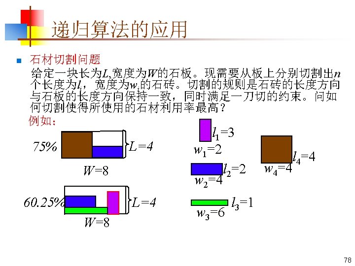
Homework n Page 48 -49 4. 3 4. 5 4. 7 4. 12 4. 15 实验4. 17 和4. 18至少 2道* 77