Technion Computer Science Department Center for Intelligent Systems

Technion - Computer Science Department Center for Intelligent Systems Person Re-Identification Application for Android Instructor: Yair Atzmon Student: Dmitry Altshuler

Introduction � Person Re-Identification related problems. is one of the security field � Person Re-Identification has few challenges Low resolution cameras Illumination changes, like Indoor and Outdoor Pose changes. Geometry changes. � A Re-Identification algorithm based on color Invariant was invented and presented in paper “Color Invariant for Person Re-Identification” By Igor Kviatkovsky, Amit Adam and Ehud Rivlin.

Algorithm Description � The input of the algorithm is an image and its silhouette. � Colorspace and Covariance data is extracted from the input. � 3 kinds of representations are extracted: Parts SC (from colorspace) Histogram (from colorspace) Covariance (from image & silhouette) � Two image’s representations are compared and a similarity is decided (similar or not)

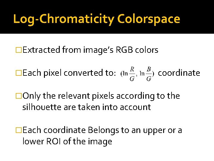
Log-Chromaticity Colorspace �Extracted from image’s RGB colors �Each pixel converted to: coordinate �Only the relevant pixels according to the silhouette are taken into account �Each coordinate Belongs to an upper or a lower ROI of the image

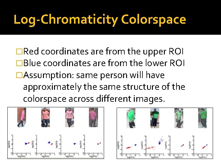
Log-Chromaticity Colorspace �Red coordinates are from the upper ROI �Blue coordinates are from the lower ROI �Assumption: same person will have approximately the same structure of the colorspace across different images.

Parts Shape Context (Parts SC) Representation �Extracted from a few sample coordinates of colorspace. From the lower and the upper ROIs of the image. �Coordinates from the lower ROI are called Reference (centers) coordinates �Coordinates from the upper ROI are called Data coordinates

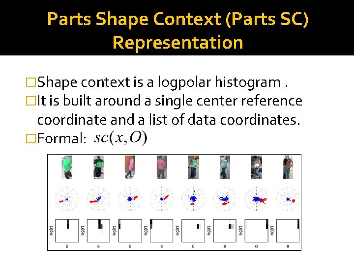
Parts Shape Context (Parts SC) Representation �Shape context is a logpolar histogram. �It is built around a single center reference coordinate and a list of data coordinates. �Formal:

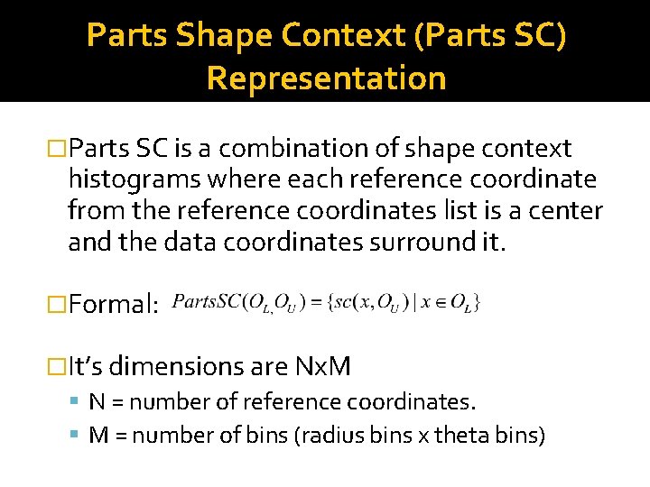
Parts Shape Context (Parts SC) Representation �Parts SC is a combination of shape context histograms where each reference coordinate from the reference coordinates list is a center and the data coordinates surround it. �Formal: �It’s dimensions are Nx. M N = number of reference coordinates. M = number of bins (radius bins x theta bins)

Comparing Parts SCs �S 1 and S 2 are two Parts SC representations. �Cost matrix – a distance matrix between every member from S 1 to every member from S 2. �The formal definition of distance between the two signatures is d(S 1 , S 2 ) = The minimal cost matching all elements in S 1 with all elements in S 2 using the cost matrix C. �To compute the minimal distance between S 1 and S 2 the EMD code is used

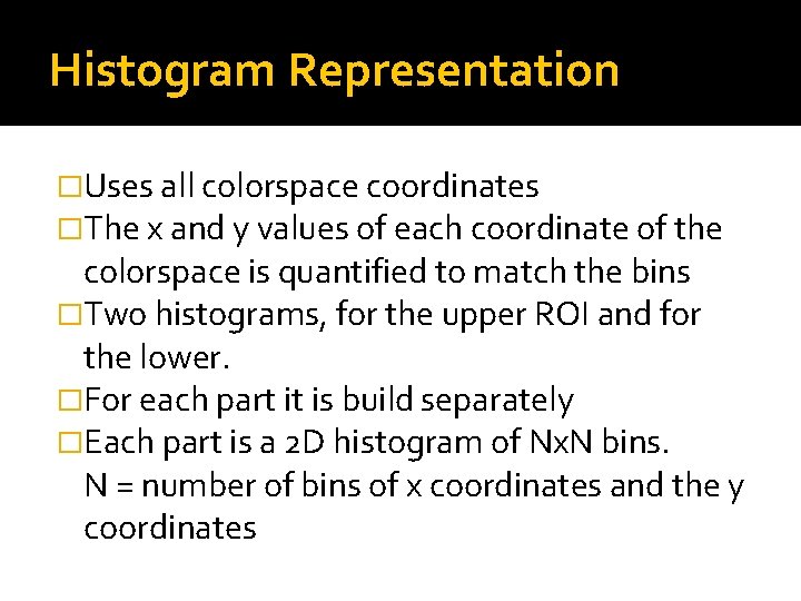
Histogram Representation �Uses all colorspace coordinates �The x and y values of each coordinate of the colorspace is quantified to match the bins �Two histograms, for the upper ROI and for the lower. �For each part it is build separately �Each part is a 2 D histogram of Nx. N bins. N = number of bins of x coordinates and the y coordinates

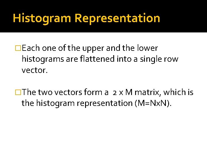
Histogram Representation �Each one of the upper and the lower histograms are flattened into a single row vector. �The two vectors form a 2 x M matrix, which is the histogram representation (M=Nx. N).

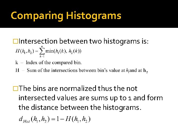
Comparing Histograms �Intersection between two histograms is: �The bins are normalized thus the not intersected values are sums up to 1 and form the distance between the histograms.

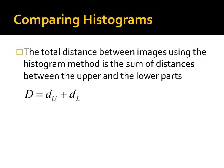
Comparing Histograms �The total distance between images using the histogram method is the sum of distances between the upper and the lower parts

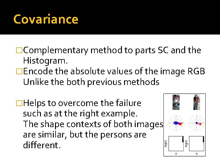
Covariance �Complementary method to parts SC and the Histogram. �Encode the absolute values of the image RGB Unlike the both previous methods �Helps to overcome the failure such as at the right example. The shape contexts of both images are similar, but the persons are different.

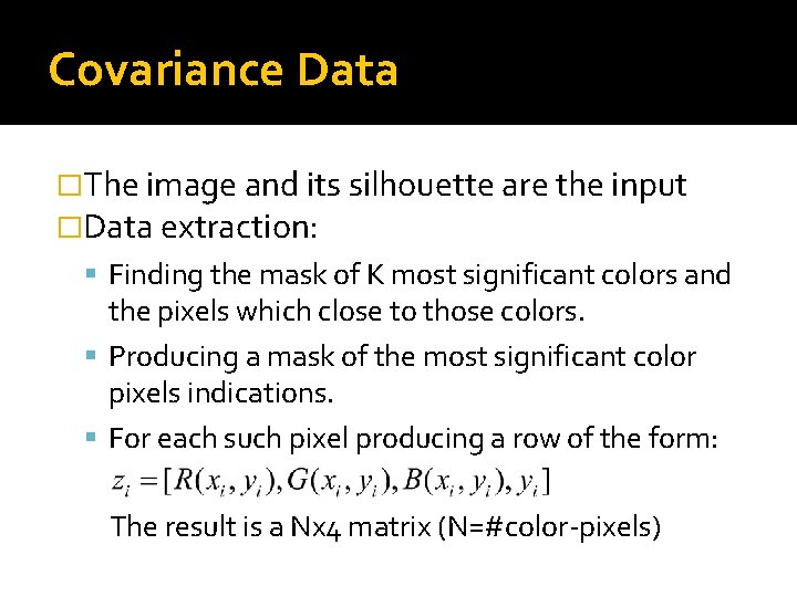
Covariance Data �The image and its silhouette are the input �Data extraction: Finding the mask of K most significant colors and the pixels which close to those colors. Producing a mask of the most significant color pixels indications. For each such pixel producing a row of the form: The result is a Nx 4 matrix (N=#color-pixels)

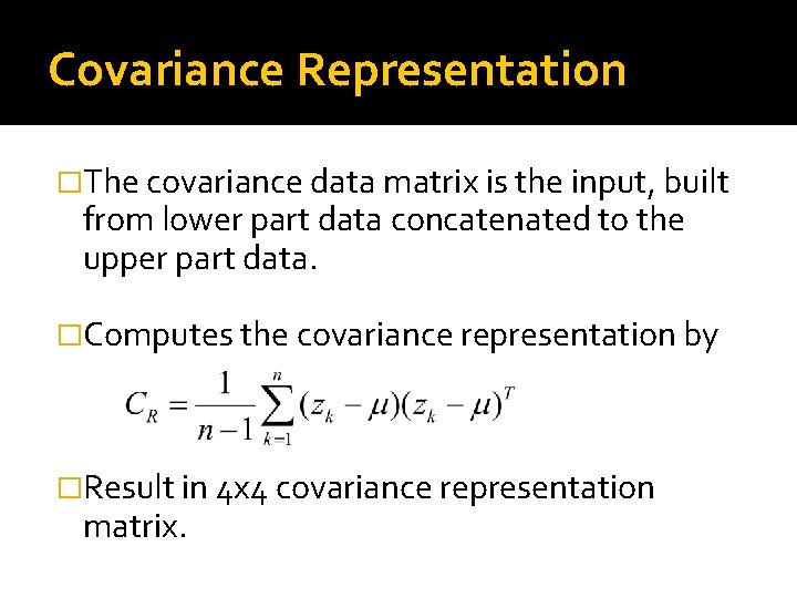
Covariance Representation �The covariance data matrix is the input, built from lower part data concatenated to the upper part data. �Computes the covariance representation by �Result in 4 x 4 covariance representation matrix.

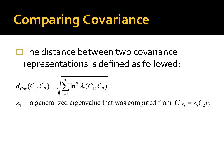
Comparing Covariance �The distance between two covariance representations is defined as followed:

Thresholds �When a distance between images is calculated it is compared it a threshold value. �When d=< th means that persons on the images are similar and d> th => they are different. �In order to define a sensible threshold some statistic was made.

Thresholds �VIPe. R database composed of 1264 images when any image has its matching image in it. �The first 632 images match the other 632 images

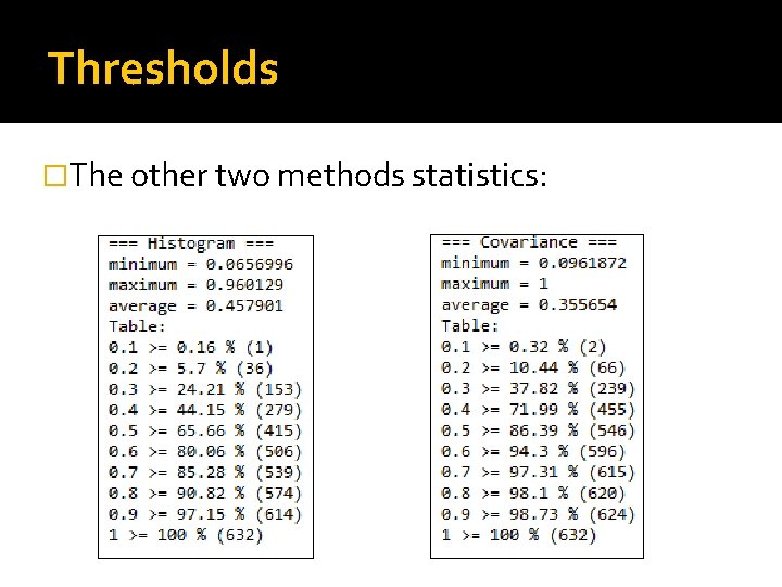
Thresholds �For every Parts SC, Histogram, and the Covariance method, computed: Average distance Minimum distance Maximum distance Table of cumulative distances �The distance that were measured were only of the correct matching images.

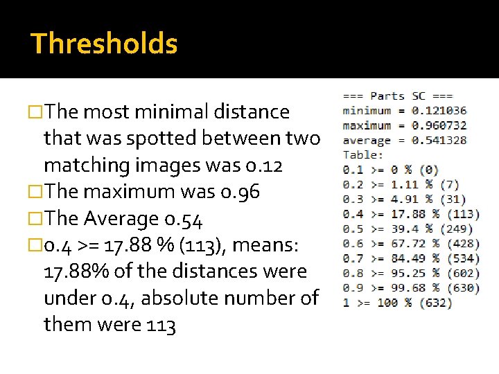
Thresholds �The most minimal distance that was spotted between two matching images was 0. 12 �The maximum was 0. 96 �The Average 0. 54 � 0. 4 >= 17. 88 % (113), means: 17. 88% of the distances were under 0. 4, absolute number of them were 113

Thresholds �The other two methods statistics:

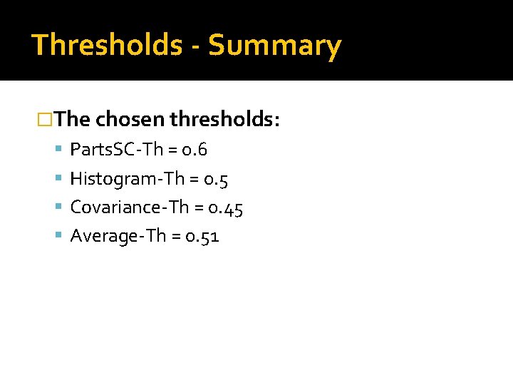
Thresholds - Summary �The chosen thresholds: Parts. SC-Th = 0. 6 Histogram-Th = 0. 5 Covariance-Th = 0. 45 Average-Th = 0. 51

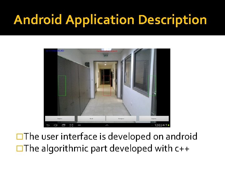
Android Application Description �The user interface is developed on android �The algorithmic part developed with c++

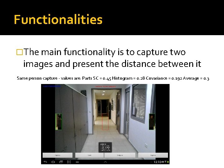
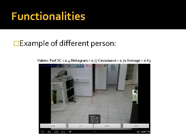
Functionalities �The main functionality is to capture two images and present the distance between it Same person capture - values are: Parts SC = 0. 45 Histogram = 0. 28 Covariance = 0. 192 Average = 0. 3

Functionalities �Example of different person: Values: Part SC = 0. 4 Histogram = 0. 77 Covariance = 0. 71 Average = 0. 63

Functionalities �The user can also send the image to a distant device and change the resolution of the camera preview. �For sending the data a communication convention was set using the xml standard

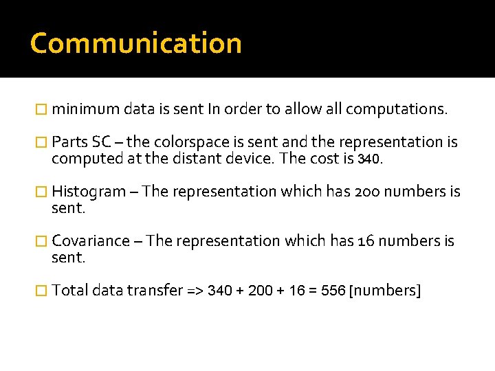
Communication �Data transfer costs: Image => 128 x 48 x 3 = 18432 [numbers] Silhouette => 128 x 48 = 6144 All colorspace => 2 x (128 x 48) = 12288 Samples of colorspace 2 x (85 x 2) = 340 Parts SC => 85 x 120 = 10200 Histogram => 2 x 100 = 200 Covariance Data => unknown x 4 Covariance Representation => 4 x 4 = 16

Communication � minimum data is sent In order to allow all computations. � Parts SC – the colorspace is sent and the representation is computed at the distant device. The cost is 340. � Histogram – The representation which has 200 numbers is sent. � Covariance – The representation which has 16 numbers is sent. � Total data transfer => 340 + 200 + 16 = 556 [numbers]

Communication �As the calculation shows, sending the representations (and the parts. SC colorspace) is much cheaper (556 numbers) than sending the original image and its silhouette (total sent of 24576 numbers). �It is actually 24576 / 556 =~ 44 times less information to send.

API Testing �The current project is based on a previous project done with Matlab. �For every API function it is tested that for the same input the functions produces the same output as in Matlab.

Conclusions �Covariance representation helps to complete the parts SC and the Histogram representations. �Using the average distance value results in a more precise conclusions. �Sending the representations is much cheaper rather than sending the original image.

Thank You