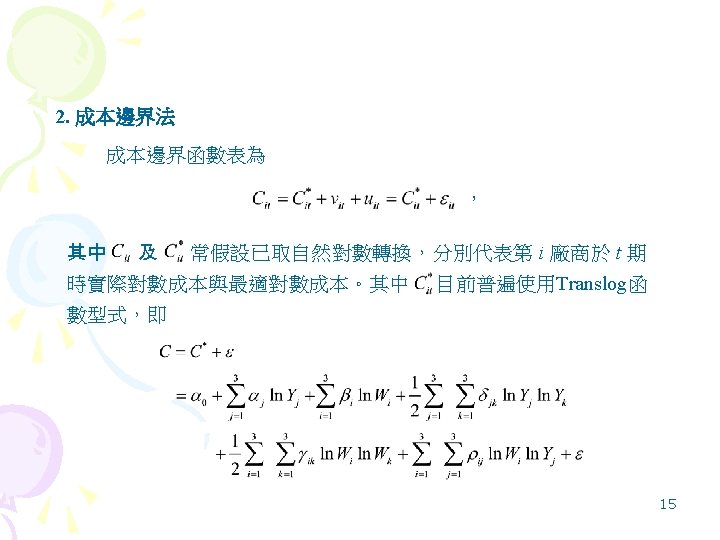
Technical efficiency Input orientation Farrel 1957 A B

 A B D C I")
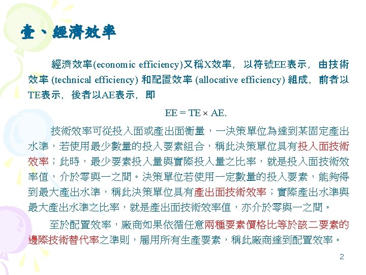
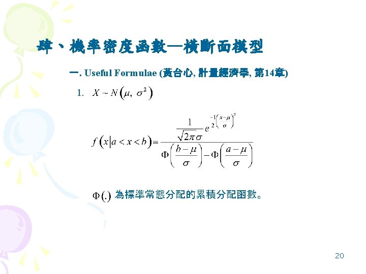
經濟的效率衡量 • Technical efficiency : Input orientation, Farrel (1957) A B D C I 1=1 0 X 1/Y – I 1: unit isoquant 單位等產量線 – I 1上各點,為最有效率的要素投入組合。 3
的衡量表為 Y Y* Y=f (X) : production frontier Output orientation A")
• 若廠商使用A點投入組合,生產一單位產出,則技術效 率(TEI)的衡量表為 Y Y* Y=f (X) : production frontier Output orientation A Input orientation 0 X CRTS TEI=TEO 4

A B D C 0 5
 shiffs to ft+1(x) Efficiency change TEt→TEt+1 50% 6")
Y 0 X Productivity Change ft(x) shiffs to ft+1(x) Efficiency change TEt→TEt+1 50% 6
 • Definition 1: An input distance function is a function L(y)")
貳、 距離函數(Distance Functions) • Definition 1: An input distance function is a function L(y) input requirement set for output y. ={x: x can produce y} Y L(y) f (X) y x x 0 L(y) X 一投入,一產出 x is feasible for y, but y can be produced with smaller input x/λ 1 and so DI(y, x)=λ 1 >1 0 X 1 二種投入 x is feasible for y, but y can be produced with the radially contracted input vector 7 x/λ 2 and so DI(y, x)=λ 2 >1
具備下述性質 1. DI(0, x)=+∞ and DI(y, 0)=0 2. DI(y, x) is")
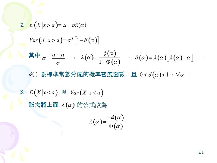
• DI(y, x)具備下述性質 1. DI(0, x)=+∞ and DI(y, 0)=0 2. DI(y, x) is an upper-semicontinuous function 3. DI(y, λx)=λDI(y, x) for λ>0 homo. of deg. 1 4. DI(y, λx)≧DI(y, x) for λ≧ 1 5. DI(λy, x)≦DI(y, x) for λ≧ 1 8

• Definition 2: An output distance function is a function describes the sets of output vectors that are feasible for each input vector , y GR 0 Y x f (X) P(x) y y 0 x (*) 一投入,一產出 X 0 兩種產出 y 1 9
具備下述性質 1. DO(0, x)=0 and DO (y, 0 )=+∞ 2. DO")
• DO(y, x)具備下述性質 1. DO(0, x)=0 and DO (y, 0 )=+∞ 2. DO (y, x) is an lower-semicontinuous function 3. DO (λy, x)=λDO (y, x) for λ>0 4. DO (y, λx) ≦ DO (y, x) for λ≧ 1 5. DO (λy, x) ≦DO(y, x) for 0≦λ≦ 1 由圖(*) DO(y, x)=y/f(x)≦ 1 (**) 10

• The relationships between distance functions and radial efficiency measures (K & L, P. 50) TEI(y, x) =[DI(y, x)]-1 and TEO(y, x) = DO(y, x). 11
 或稱無母數法 資料包絡分析法 (data envelopment analysis),簡稱 DEA。 三. 半參數法 (semi-parametric approach) 或稱半母數法 1. Nonparametric Regression")
二. 無參數法 (nonparametric approach) 或稱無母數法 資料包絡分析法 (data envelopment analysis),簡稱 DEA。 三. 半參數法 (semi-parametric approach) 或稱半母數法 1. Nonparametric Regression (Fan, Li, and Weersink, 1996, JBES) 2. Semi-parametric Regression (1) Partially Linear Model (2) Fourier Flexible Functional Form (Mitchell and Onvural, 1996, JMCB, Ivaldi et al. , 1996, JAE, Huang and Wang, 2004, JPA) 3. Semi-parametric Smooth Coefficient Model (Li et al. , 2002, JBES) 19

二. Half-Normal Distribution and are independent. 23

24
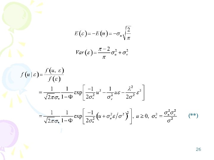
 is the density function variable truncated")
除 項以外,其他各項為 的隨機變數, , of a , 。(**) is the density function variable truncated at zero from below. or 27
 建議 由(*),對數概似函數可表為 n: sample size The parameter")
Battese and Coelli (1988, J. of Econometrics) 建議 由(*),對數概似函數可表為 n: sample size The parameter estimates are consistent as . 28

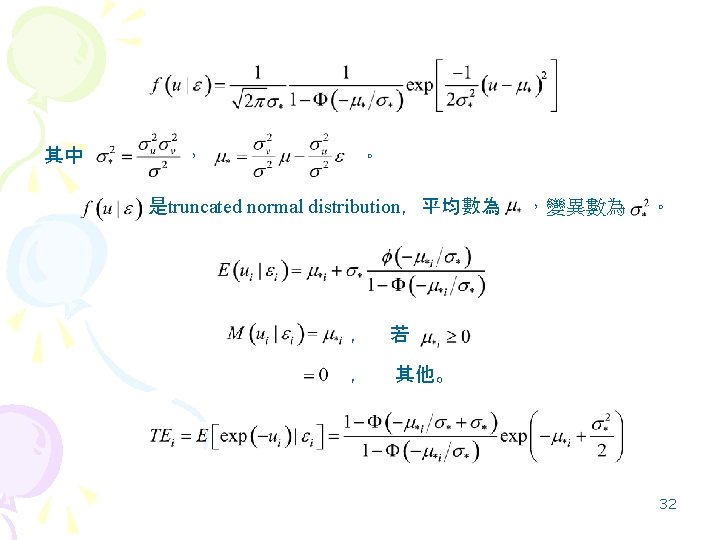
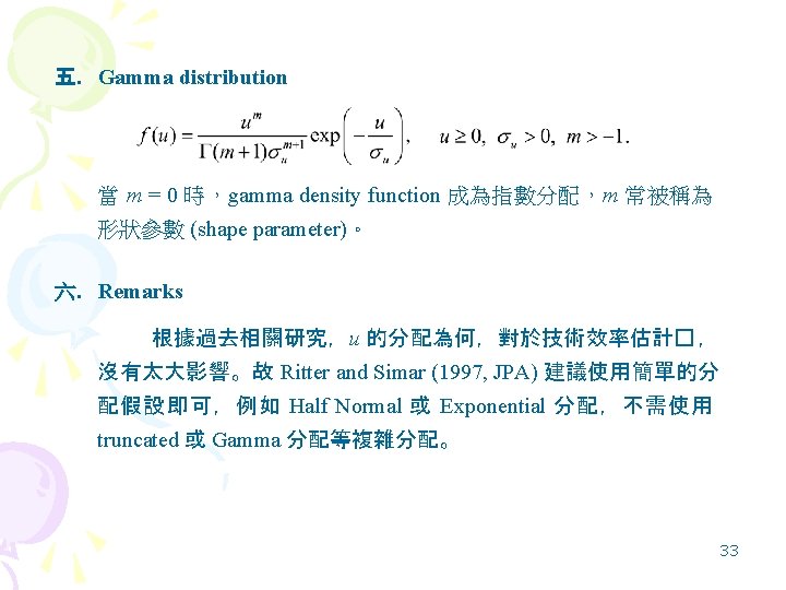
三. Exponential distribution 是truncated normal distribution,平均數為 ,變異數為 。 29

30

四. Truncated normal distribution 其中 , 。 31
 一. Time Invariant Technical Efficiency 代表 time-invariant production inefficiency, 可 視")
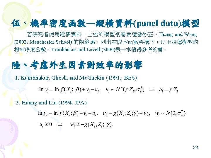
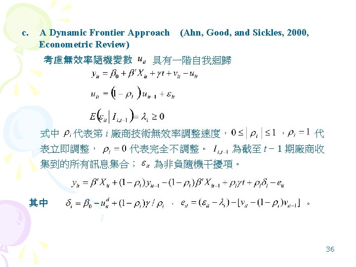
柒、無分配法(distribution-free approach) 一. Time Invariant Technical Efficiency 代表 time-invariant production inefficiency, 可 視 為 固 定 效 果 (fixed-effects)或 隨 機 效 果 (randomeffects)。 二. Time Variant Technical Efficiency (1) Lee and Schmidt (1993): 是一組時間虛擬變數。 (2) Kumbhakar (1990): (3) Battese and Coelli (1992): 35
 TSP(http: //www. tspintl. com) Stata GAUSS Frontier 4. 1 37")
捌、套裝軟體簡介 Limdep (Frontier指令) TSP(http: //www. tspintl. com) Stata GAUSS Frontier 4. 1 37
, Modeling allocative inefficiency in a translog cost function")
玖、配置效率 1. Kumbhakar, S. C. (1997), Modeling allocative inefficiency in a translog cost function and cost share equations: An exact relationship, Journal of Econometrics, 76, 351 -356. 2. Kumbhakar, S. C. and H. J. Wang (2006), Estimation of technical and allocative inefficiency: A primal system approach, Journal of Econometrics, 134, 419 -440. 3. Atkinson, S. E. and C. Cornwell (1994), Parametric estimation of technical and allocative inefficiencies with panel data, International Economic Review, 35, 231 -243. 4. 黃台心 (1999), 由利潤函數衡量我國銀行廠商之經濟效率 ---- 參數計 量法的應用,中央研究院經濟研究所,經濟論文,第二十七卷,第 二期,283 -309。 38
 Reference: Kumbhakar and Lovell (2000) Chapter 8 50")
拾壹、總要素生產力(Total Factor Productivity, TFP) Reference: Kumbhakar and Lovell (2000) Chapter 8 50
 •")
• We start with the deterministic production frontier • (8. 2. 1) • Where y is the scalar output of a producer, is the deterministic kernel of a stochastic production frontier with technology parameter vector to be estimated, is an input vector, t is a time trend serving as a proxy for technical change, and represents outputoriented technical inefficiency. Technical change is not restricted to be neutral with respect to the inputs; neutrality requires that 51

In the scalar output case a conventional Divisia index of productivity change is defined as the difference between the rate of change of output and the rate of change of an input quantity index, and so (8. 2. 4) where a dot over a variable indicates its rate of change is the observed expenditure share of input is total expenditure, and is an input price vector. 52

• A measure of the rate of technical change • A measure of the rate of change in technical efficiency 53
 and inserting the resulting expression for into equation")
Totally differentiating equation (8. 2. 1) and inserting the resulting expression for into equation (8. 2. 4) yields (8. 2. 5) where are elasticities of output with respect to each of the inputs. The scale elasticity provides a primal measure of returns to scale characterizing the production frontier. 54
 decomposes productivity change into four components a")
The relationship in equation (8. 2. 5) decomposes productivity change into four components a technical change component a scale component a technical efficiency change component an allocative inefficiency component This decomposition of productivity change is very similar to the decomposition obtained by Bauer (1990, JPA). 55
- Slides: 55