Team Kenya Outline 1 2 3 4 5

Team Kenya

Outline 1. 2. 3. 4. 5. Lessons learnt Case of Kenya: Overview Test for Stationarity of CPI variable VAR analysis Policy insights

1. Lessons Learnt • How to test for stationarity using appropriate models, that is, testing for validity of including trend and/or constant term. • Testing for stability / stationarity of a VAR model. • How to use Eviews. • How to interpret impulse response functions.

2. Case of Kenya: Overview • Study period 2000: 1 to 2013: 3 • Data source: Central Bank of Kenya and Kenya National Bureau of Statistics • Frequency of data: Quarterly • Variables: CPI, M 3, RGDP, TB 3, e, libor, oilprice • Methodology: Granger causality, Johansen cointegration test, impulse response analysis

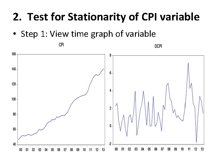
2. Test for Stationarity of CPI variable • Step 1: View time graph of variable

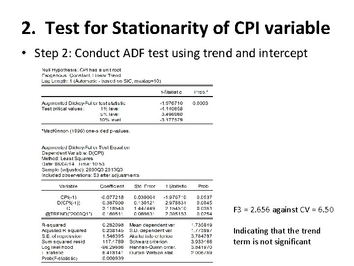
2. Test for Stationarity of CPI variable • Step 2: Conduct ADF test using trend and intercept F 3 = 2. 656 against CV = 6. 50 Indicating that the trend term is not significant

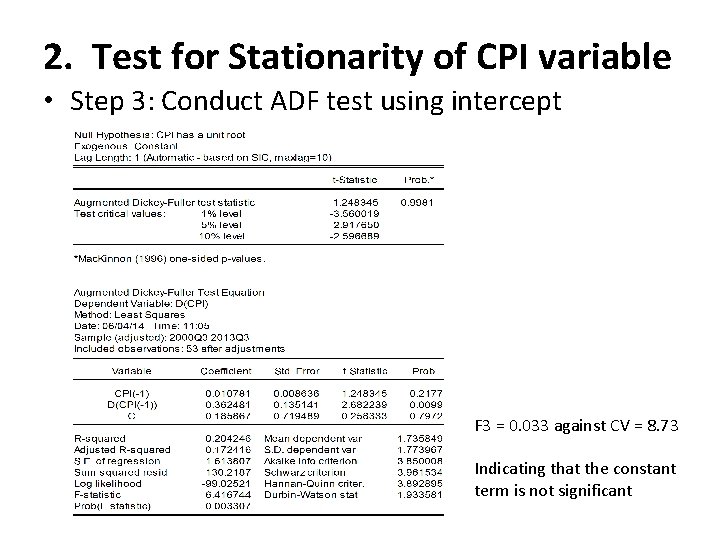
2. Test for Stationarity of CPI variable • Step 3: Conduct ADF test using intercept F 3 = 0. 033 against CV = 8. 73 Indicating that the constant term is not significant

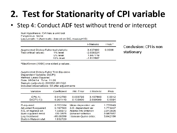
2. Test for Stationarity of CPI variable • Step 4: Conduct ADF test without trend or intercept Conclusion: CPI is non stationary

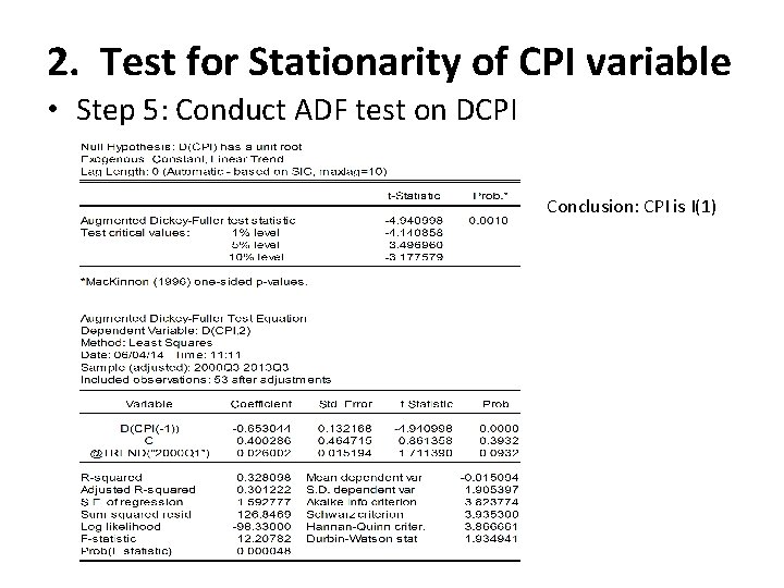
2. Test for Stationarity of CPI variable • Step 5: Conduct ADF test on DCPI Conclusion: CPI is I(1)

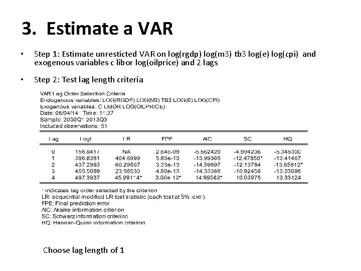
3. Estimate a VAR • Step 1: Estimate unresticted VAR on log(rgdp) log(m 3) tb 3 log(e) log(cpi) and exogenous variables c libor log(oilprice) and 2 lags • Step 2: Test lag length criteria Choose lag length of 1

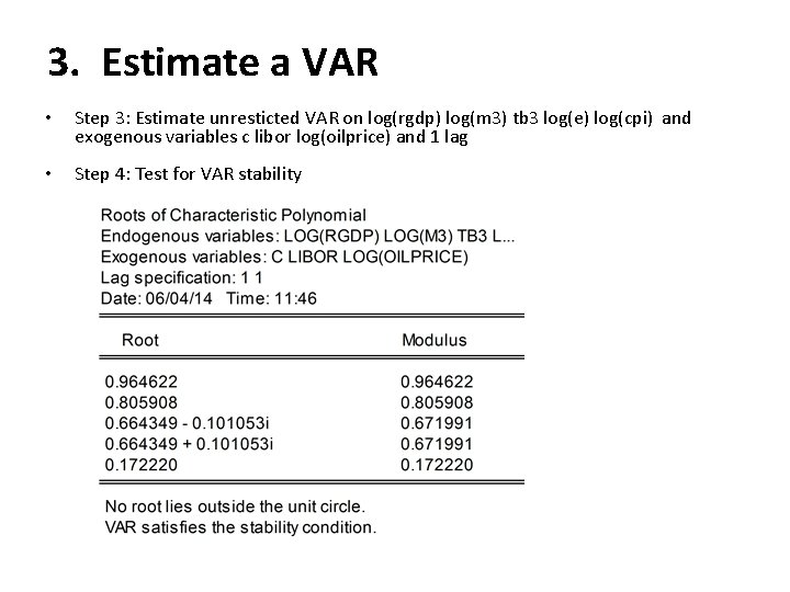
3. Estimate a VAR • Step 3: Estimate unresticted VAR on log(rgdp) log(m 3) tb 3 log(e) log(cpi) and exogenous variables c libor log(oilprice) and 1 lag • Step 4: Test for VAR stability

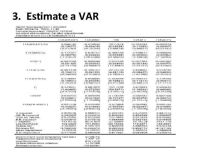
3. Estimate a VAR

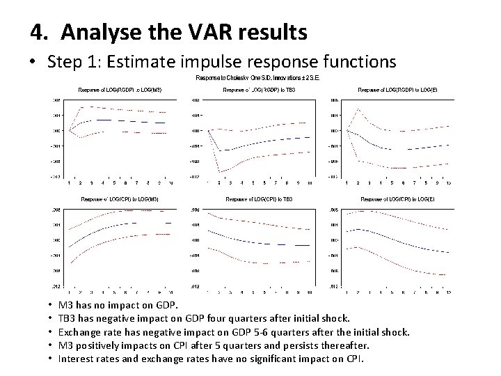
4. Analyse the VAR results • Step 1: Estimate impulse response functions • • • M 3 has no impact on GDP. TB 3 has negative impact on GDP four quarters after initial shock. Exchange rate has negative impact on GDP 5 -6 quarters after the initial shock. M 3 positively impacts on CPI after 5 quarters and persists thereafter. Interest rates and exchange rates have no significant impact on CPI.

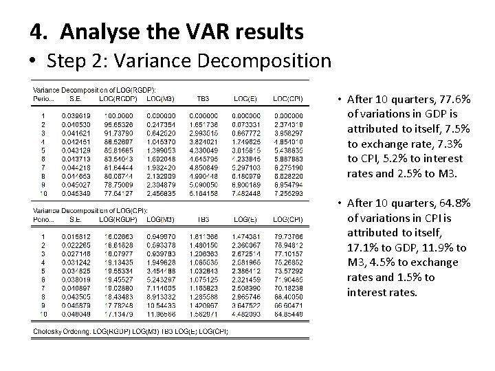
4. Analyse the VAR results • Step 2: Variance Decomposition • After 10 quarters, 77. 6% of variations in GDP is attributed to itself, 7. 5% to exchange rate, 7. 3% to CPI, 5. 2% to interest rates and 2. 5% to M 3. • After 10 quarters, 64. 8% of variations in CPI is attributed to itself, 17. 1% to GDP, 11. 9% to M 3, 4. 5% to exchange rates and 1. 5% to interest rates.

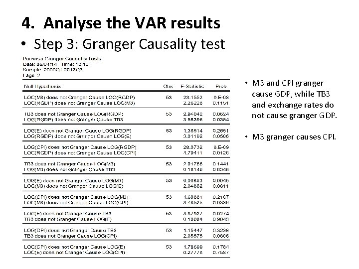
4. Analyse the VAR results • Step 3: Granger Causality test • M 3 and CPI granger cause GDP, while TB 3 and exchange rates do not cause granger GDP. • M 3 granger causes CPI.

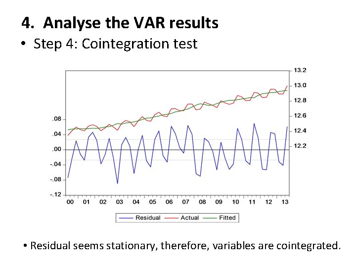
4. Analyse the VAR results • Step 4: Cointegration test • Residual seems stationary, therefore, variables are cointegrated.

5. Policy insights • Excessive money is not good for inflation in the medium-term. • Raising short-term interest rates and depreciating the shilling will impact negatively on growth in the short term.

• Thank you for listening