Tabular Methods Statistical Tables 1 1 Tabular Methods

Tabular Methods (Statistical Tables ) 1 1

Tabular Methods (Statistical Tables ) • A statistical table is an orderly and systematic presentation of numerical data in rows and columns. • Rows (stubs) are horizontal and columns (captions) are vertical arrangements. • The use of tables for organizing data involves grouping the data into mutually exclusive categories of the variables and counting the number of occurrences (frequency) to each category. 2 2

Tabular presentation cont… • Almost any form of quantitative or qualitative data can be organized by tables • Uses • To demonstrate patterns, differences and other relationships • Serve as the basis for preparing more visual displays of data, such as graphs and charts, where some of the detail may be lost • A statistical table has at least four major parts and some other minor parts 3 1. The Title 2. Column 3. Row 4. The Body 5. Prefatory Notes , Foots Notes , Source Notes…. 3

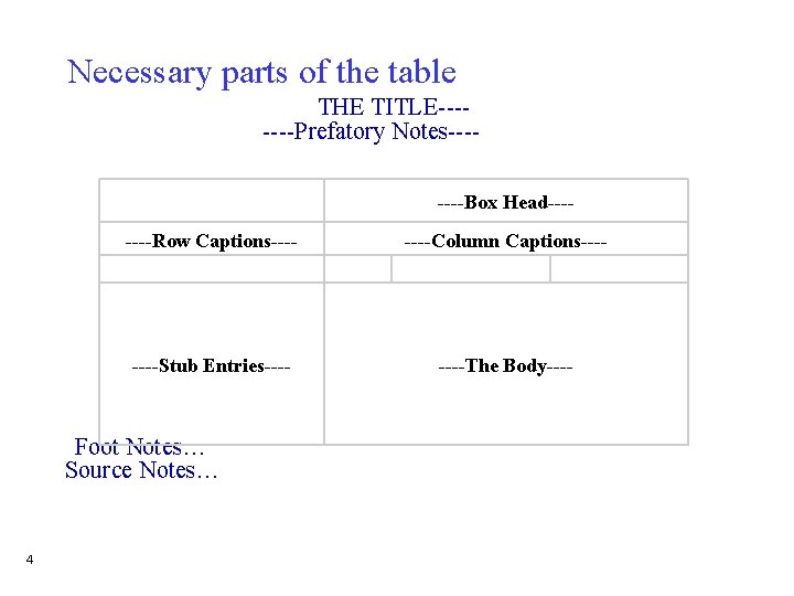
Necessary parts of the table THE TITLE-------Prefatory Notes--- ----Box Head-------Row Captions---- ----Column Captions--- ----Stub Entries---- ----The Body---- Foot Notes… Source Notes… 4 4

Guidelines for constructing tables 5 • Keep them simple, • All tables should be self-explanatory, • Include clear title telling what, when and where, • Clearly label the rows and columns, • State clearly the unit of measurement used, • Explain codes and abbreviations in the foot-note, • Show totals, • Numerical entities of zero should be explicitly written rather than indicated by a dash (missing value) • If data is not original, indicate the source in footnote. 5

Based on the purpose for which the table is designed and the complexity of the relationship, a table could be: 1. Simple or one way table: 2. Two-way table: 3. Higher Order Table: A. Simple or one way table: • • 6 Is used when the individual observations involve only to a single variable. The denominators for the percentages are the sum of all observed frequencies. 6

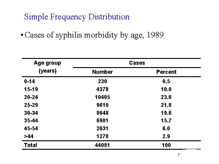
Simple Frequency Distribution • Cases of syphilis morbidity by age, 1989 Age group (years) Cases Number Percent 0 -14 15 -19 20 -24 25 -29 30 -34 35 -44 45 -54 >44 230 4378 10405 9610 8648 6901 2631 1278 0. 5 10. 0 23. 6 21. 8 19. 6 15. 7 6. 0 2. 9 Total 44081 100 7 7

B. Two-way table: • Shows two characteristics and • Is formed when either the caption or the stub is divided into two parts. • • 8 The cross tabulation is used to obtain the frequency distribution of one variable by the subset of another variable. The decision for the denominator is based on the variable of interest to be compared over the subset of the other variable. 8

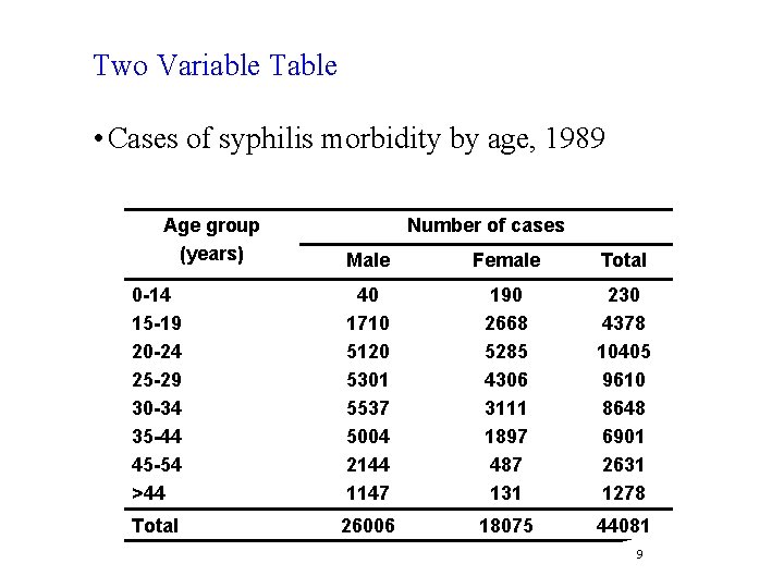
Two Variable Table • Cases of syphilis morbidity by age, 1989 Age group (years) Number of cases Male Female Total 0 -14 15 -19 20 -24 25 -29 30 -34 35 -44 45 -54 >44 40 1710 5120 5301 5537 5004 2144 1147 190 2668 5285 4306 3111 1897 487 131 230 4378 10405 9610 8648 6901 2631 1278 Total 26006 18075 44081 9 9

C. Higher Order Table • When it is desired to represent three or more characteristics in a single table. Example • If it is desired to represent the `Profession, ' `sex' and `Residence, ' of the study individuals. 1 0 10

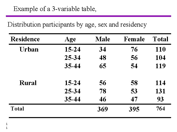
Example of a 3 -variable table, Distribution participants by age, sex and residency Residence Male Female Total Urban 15 -24 25 -34 35 -44 34 48 65 76 56 54 110 104 119 Rural 15 -24 25 -34 35 -44 56 78 46 369 58 53 47 395 114 131 93 Total 1 1 Age 764 11

Composite tables • It is a large table combining several separate tables • Age, sex and other demographic variables may be combined to form a single table 1 2 12

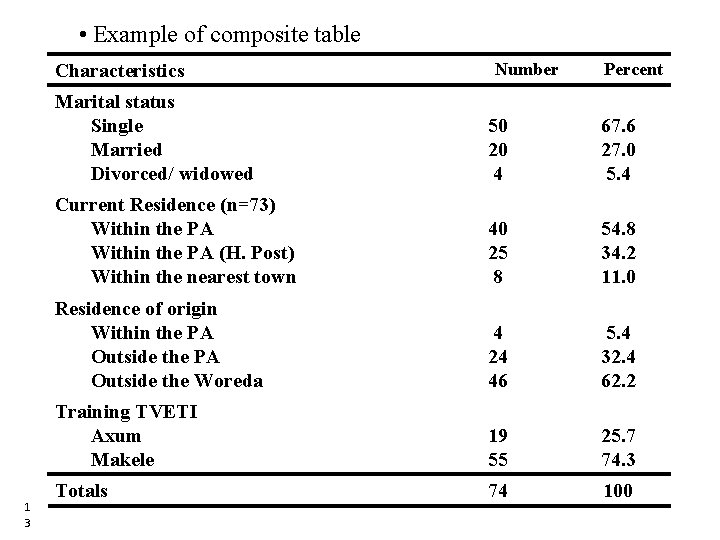
• Example of composite table Characteristics 1 3 Number Percent Marital status Single Married Divorced/ widowed 50 20 4 67. 6 27. 0 5. 4 Current Residence (n=73) Within the PA (H. Post) Within the nearest town 40 25 8 54. 8 34. 2 11. 0 Residence of origin Within the PA Outside the Woreda 4 24 46 5. 4 32. 4 62. 2 Training TVETI Axum Makele 19 55 25. 7 74. 3 Totals 74 100 13

Graphical Methods ( Diagrammatic Representation of Data) 1 4 14

Graphical Methods ( Diagrammatic Representation of Data) • Appropriately drawn graph allows readers to obtain rapidly an overall grasp of the data presented. • The relationship between numbers of various magnitudes can usually be seen more quickly and easily from a graph than from a table. • They are probably simpler and more easily understandable. • It consists in presenting statistical material in pictures, maps and lines or curves. 1 5 15

Importance of Diagrammatic Representation üHave greater attraction than mere figures. üHelp in deriving the required information in less time and without any mental strain. üFacilitate comparison. üReveal unsuspected patterns in a complex set of data and may suggest directions in which changes are occurring. üHave greater memorizing value than mere figures. 1 6 16

Limitations of Diagrammatic Representation ØThe technique is made use only for purposes of comparison. It is not to be used when comparison is either not possible or is not necessary. Ø is not an alternative to tabulation. It only strengthens the textual exposition of a subject, and cannot serve as a complete substitute for statistical data. ØIt can give only an approximate idea and as such where greater accuracy is needed diagrams will not be suitable. ØThey fail to bring to light small differences 1 7 17

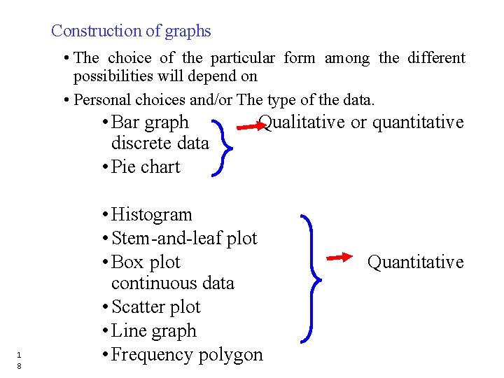
Construction of graphs • The choice of the particular form among the different possibilities will depend on • Personal choices and/or The type of the data. • Bar graph Qualitative or quantitative discrete data • Pie chart 1 8 • Histogram • Stem-and-leaf plot • Box plot Quantitative continuous data • Scatter plot • Line graph • Frequency polygon 18

General rules that are commonly accepted about construction of graphs: - . Every graph should be self-explanatory and as simple as 1 possible. 2. Titles are usually placed below the graph and it should again question what ? Where? When? How classified? 3. Legends or keys should be used to differentiate variables if more than one is shown. 4. The axes label should be placed to read from the left side and from the bottom. 5. The units in to which the scale is divided should be clearly indicated. 6. The numerical scale representing frequency must start at zero or a break in the line should be shown. 1 9 19

1. Bar Chart • Used to represent and compare the frequency distribution of discrete variables and attributes or categorical series. • All the bars must have equal width and the distance between bars must be equal. • Label both axes clearly and All the bars should rest on the same line called the base. • There are different types of bar diagrams, depending on the objective and type of information that we want to present. • The most important ones are üSimple bar chart üMultiple bar chart üComponent bar chart ( actual and percentage ) 2 0 20

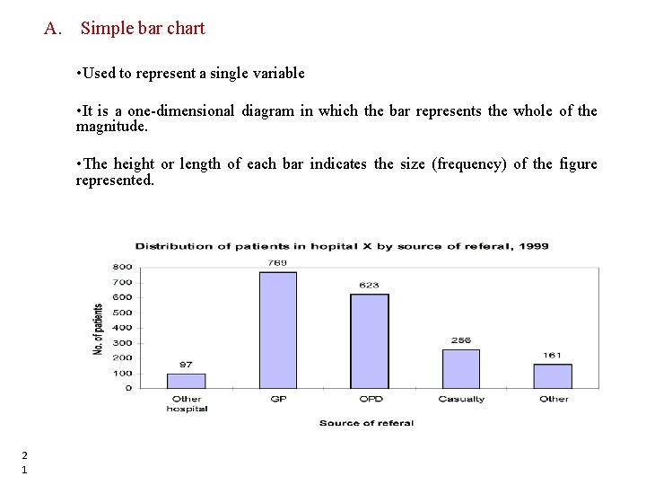
A. Simple bar chart • Used to represent a single variable • It is a one-dimensional diagram in which the bar represents the whole of the magnitude. • The height or length of each bar indicates the size (frequency) of the figure represented. 2 1 21

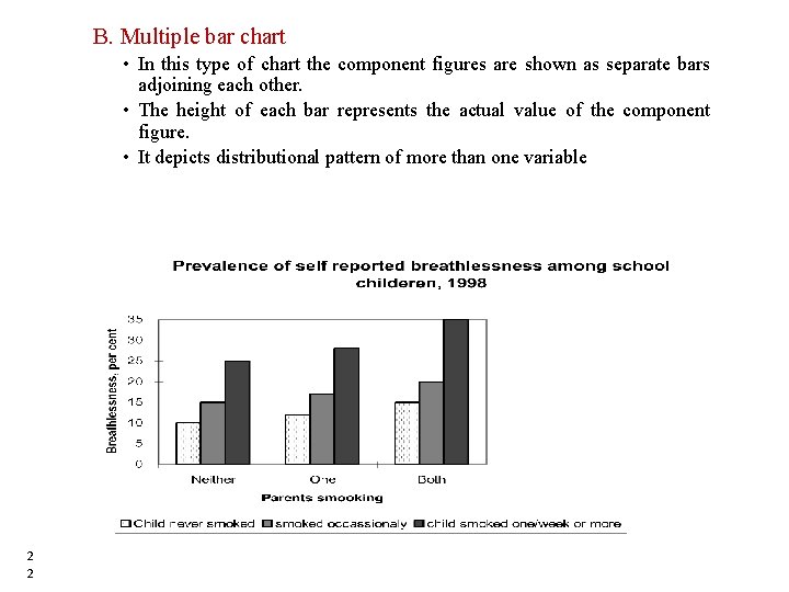
B. Multiple bar chart • In this type of chart the component figures are shown as separate bars adjoining each other. • The height of each bar represents the actual value of the component figure. • It depicts distributional pattern of more than one variable 2 2 22

C. Component (or sub-divided) Bar Diagram • • Bars are sub-divided into component parts of the figure. These sorts of diagrams are constructed when each total is built up from two or more component figures. They can be of two kind: I. Actual Component Bar Diagrams When the over all height of the bars and the individual component lengths represent actual figures. • II. Percentage Component Bar Diagram • Where the individual component lengths represent the percentage each component forms the over all total. • A series of such bars will all be the same total height, i. e. , 100 percent. 2 3 23

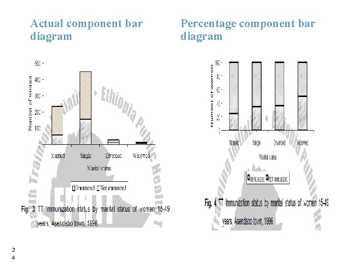
Actual component bar diagram 2 4 Percentage component bar diagram 24

2. Pie chart • It is a circle ( pie shaped) divided into sectors so that the areas of the sectors are proportional to the frequencies. • A good method of representation if you wish to compare a part of a group with the whole group. • The number of categories should not be too much. • Used for a single categorical variable • Use percentage distributions 2 5 25

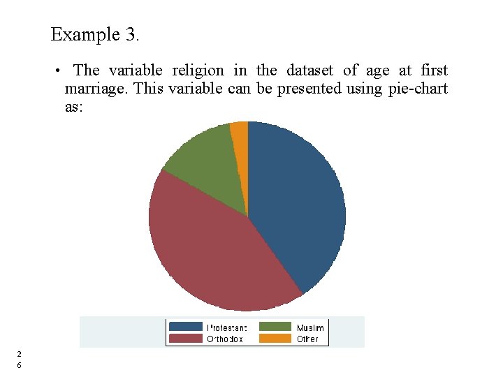
Example 3. • The variable religion in the dataset of age at first marriage. This variable can be presented using pie-chart as: 2 6 26

3. Histogram • Is the graph of the frequency distribution or relative frequency distribution of continuous or discrete measurement variables. • They are perhaps the most frequently used graphical summary for quantitative data • They describe the overall distribution shape: ØUnimodal , bimodal, or multi-modal ØBell-shaped, left-skewed, right skewed ØRange or spread of data ØAllow finding of proportions ØBars are connected (implies continuity for continuous data) ØStrictly speaking the area of each histogram bar is equal to the proportion of observations falling in an interval 27

It is constructed on the basis of the following principles a) The horizontal axis is a continuous scale running from one extreme end of the distribution to the other. It should be labeled with the name of the variable and the units of measurement. b) For each class in the distribution a vertical rectangle is drawn with (i) 2 8 Its base on the horizontal axis extending from one class boundary of the class to the other class boundary, there will never be any gap between the histogram rectangles. (ii) The bases of all rectangles will be determined by the width of the class intervals. If a distribution with unequal class-interval is to be presented by means of a histogram, it is necessary to make adjustment for varying magnitudes of the class intervals. 28

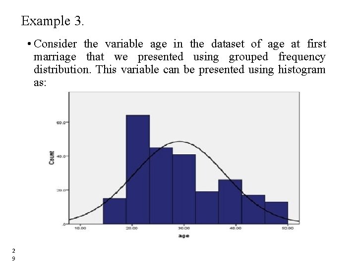
Example 3. • Consider the variable age in the dataset of age at first marriage that we presented using grouped frequency distribution. This variable can be presented using histogram as: 2 9 29

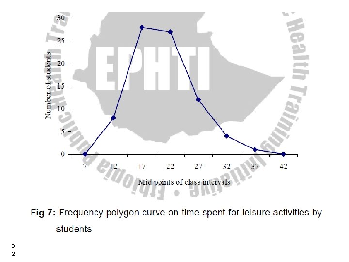
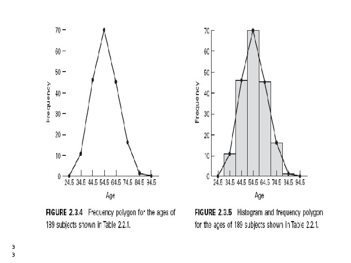
4. Frequency Polygon • If we join the midpoints of the tops of the adjacent rectangles of the histogram with line segments a frequency polygon is obtained. • When the polygon is continued to the X-axis just out side the range of the lengths the total area under the polygon will be equal to the total area under the histogram. • It is not essential to draw histogram in order to obtain frequency polygon. 3 0 30

• It can be drawn with out erecting rectangles of histogram as follows: 3 1 1. The scale should be marked in the numerical values of the midpoints of intervals. 2. Erect ordinates on the midpoints of the interval - the length or altitude of an ordinate representing the frequency of the class on whose mid-point it is erected. 3. Join the tops of the ordinates and extend the connecting lines to the scale of sizes. 31

3 2 32

3 3 33

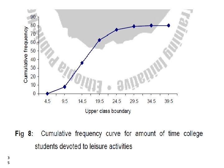
5. O give or Cumulative frequency curve • When the cumulative frequencies of a distribution are graphed the resulting curve is called O give Curve. To construct an O give curve i. Compute the cumulative frequency of the distribution. ii. Prepare a graph with the cumulative frequency on the vertical axis and the true upper class limits (class boundaries) of the interval scaled along the X-axis (horizontal axis). • The true lower limit of the lowest class interval with lowest scores is included in the X-axis scale; 3 4 34

3 5 35

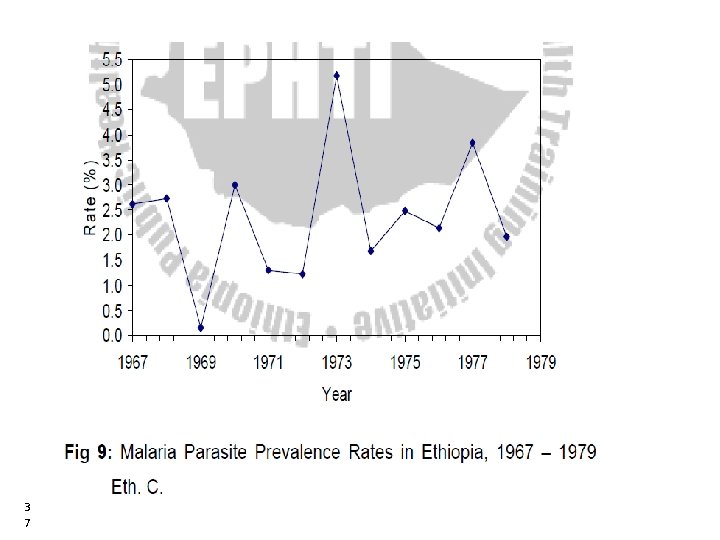
6. Line diagram • The line graph is especially useful for the study of some variables according to the passage of time. • The time, in weeks, months or years is marked along the horizontal axis; and the value of the quantity that is being studied is marked on the vertical axis. • The distance of each plotted point above the base-line indicates its numerical value. • It is suitable for depicting consecutive trend of a series over a long period. 3 6 36

3 7 37

7. Stem-and-leaf plot • Stem-and-leaf plots are a method for showing the frequency with which certain classes of values occur. • The "stem" is the left-hand column which contains the tens digits. • The "leaves" are the lists in the right-hand column, showing all the ones digits for each of the tens, twenties, thirties, and forties. • The horizontal leaves in the stem-and-leaf plot correspond to the vertical bars in the histogram, and • The leaves have lengths that equal the numbers in the frequency table. 3 8 38

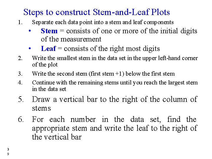
Steps to construct Stem-and-Leaf Plots 1. Separate each data point into a stem and leaf components • • 2. 3. 4. Stem = consists of one or more of the initial digits of the measurement Leaf = consists of the right most digits Write the smallest stem in the data set in the upper left-hand corner of the plot Write the second stem (first stem +1) below the first stem Continue with the remaining stems until you reach the largest stem in the data set 5. Draw a vertical bar to the right of the column of stems 6. For each number in the data set, find the appropriate stem and write the leaf to the right of the vertical bar 3 9 39

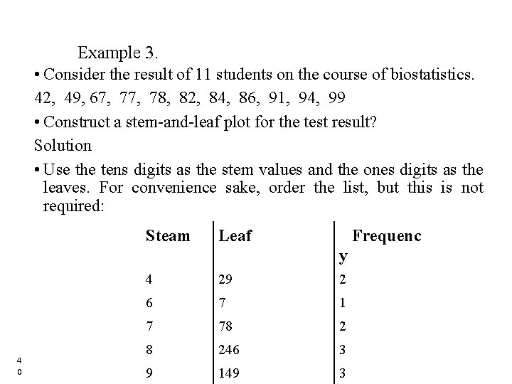
Example 3. • Consider the result of 11 students on the course of biostatistics. 42, 49, 67, 78, 82, 84, 86, 91, 94, 99 • Construct a stem-and-leaf plot for the test result? Solution • Use the tens digits as the stem values and the ones digits as the leaves. For convenience sake, order the list, but this is not required: 4 0 Steam Leaf Frequenc y 4 29 2 6 7 1 7 78 2 8 246 3 9 149 3 40

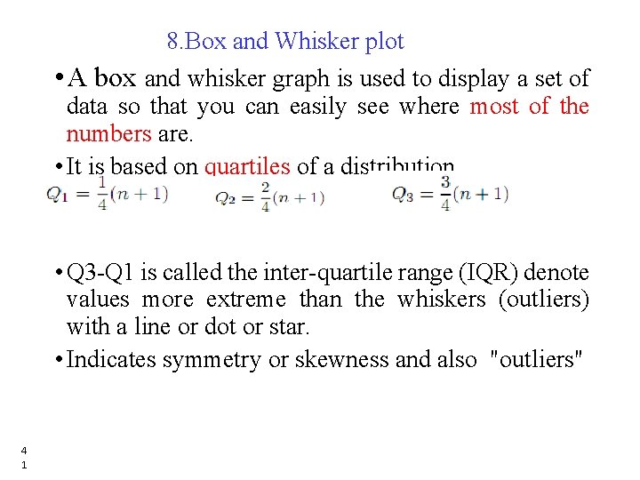
8. Box and Whisker plot • A box and whisker graph is used to display a set of data so that you can easily see where most of the numbers are. • It is based on quartiles of a distribution. • Q 3 -Q 1 is called the inter-quartile range (IQR) denote values more extreme than the whiskers (outliers) with a line or dot or star. • Indicates symmetry or skewness and also "outliers" 4 1 41

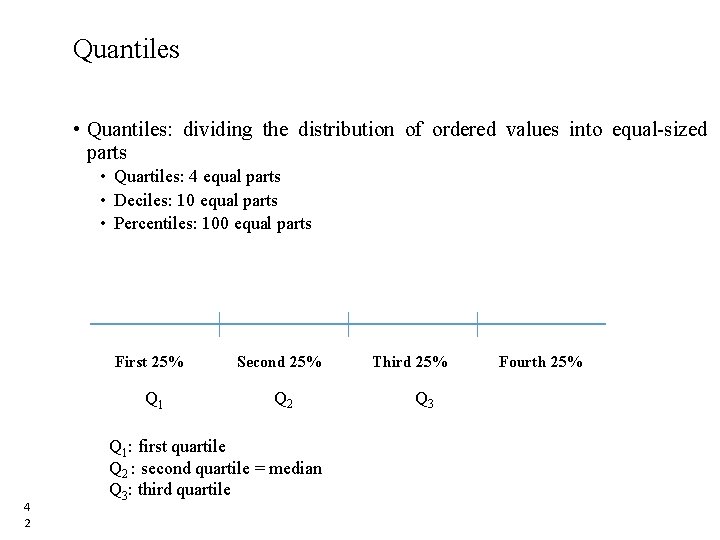
Quantiles • Quantiles: dividing the distribution of ordered values into equal-sized parts • Quartiles: 4 equal parts • Deciles: 10 equal parts • Percentiles: 100 equal parts First 25% Q 1 4 2 Second 25% Q 2 Third 25% Fourth 25% Q 3 Q 1: first quartile Q 2 : second quartile = median Q 3: third quartile 42

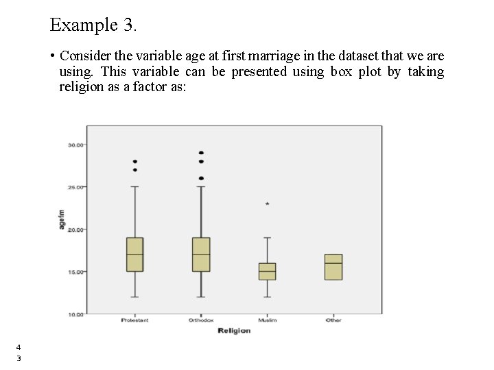
Example 3. • Consider the variable age at first marriage in the dataset that we are using. This variable can be presented using box plot by taking religion as a factor as: 4 3 43

9. Scatter Plot • Scatter plots are similar to line graphs in that they use horizontal and vertical axes to plot data points. • Scatter plots show much one variable is affected by another. 4 4 44

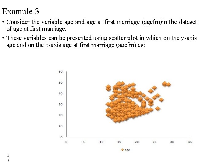
Example 3 • Consider the variable age and age at first marriage (agefm)in the dataset of age at first marriage. • These variables can be presented using scatter plot in which on the y-axis age and on the x-axis age at first marriage (agefm) as: 4 5 45