T 305 DIGITAL COMMUNICATIONS T 305 Digital Communications

T 305: DIGITAL COMMUNICATIONS T 305: Digital Communications Block II – Modelling Activities Probability & Reliability Arab Open University-Lebanon Tutorial 7 1

T 305: DIGITAL COMMUNICATIONS Introduction: Probability and Reliability used in communication Technology (e. g. Network Traffic) n The various topics covered n. Topic 1: Probability n. Topic 2: Reliability n. Topic 3: Preparation for Next Tutorial n Arab Open University-Lebanon Tutorial 7 2

T 305: DIGITAL COMMUNICATIONS Topic 1: Probability If a process or measurement can have more than one outcome, then the frequency of the ith possible outcome, referred to as the occurrence of event Ei, is the number of times, Ni, that Ei occurs out of a total number, N, of events. The value of Ni may vary each time the experiment is repeated. n Example of Ei are bits in error arrived at communication channel n The frequency of occurrence of an event may be expressed as a fraction of the total number of events. This is called a relative frequency, and the relative frequency of event Ei is given by Ni /N. n Arab Open University-Lebanon Tutorial 7 3

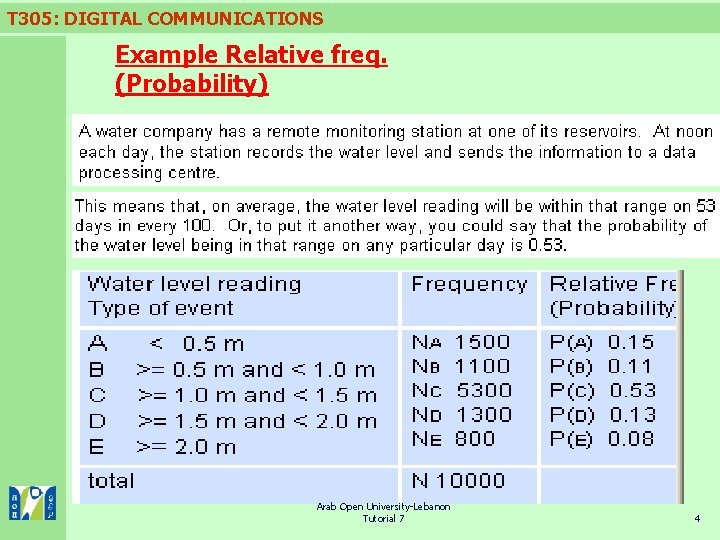
T 305: DIGITAL COMMUNICATIONS Example Relative freq. (Probability) Arab Open University-Lebanon Tutorial 7 4

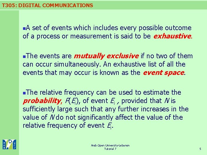
T 305: DIGITAL COMMUNICATIONS A set of events which includes every possible outcome of a process or measurement is said to be exhaustive. n The events are mutually exclusive if no two of them can occur simultaneously. An exhaustive list of all the events that may occur is known as the event space. n The relative frequency can be used to estimate the probability, P(Ei), of event Ei , provided that N is sufficiently large such that any further increases in the value of N do not significantly affect the value of the relative frequency of event Ei. n Arab Open University-Lebanon Tutorial 7 5

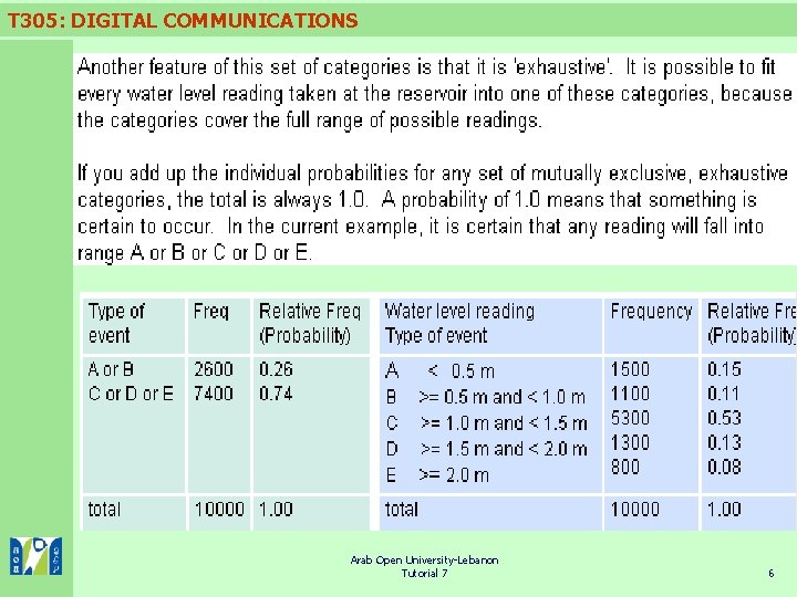
T 305: DIGITAL COMMUNICATIONS Arab Open University-Lebanon Tutorial 7 6

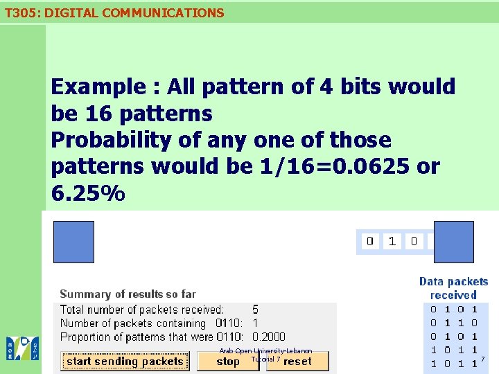
T 305: DIGITAL COMMUNICATIONS Example : All pattern of 4 bits would be 16 patterns Probability of any one of those patterns would be 1/16=0. 0625 or 6. 25% Arab Open University-Lebanon Tutorial 7 7

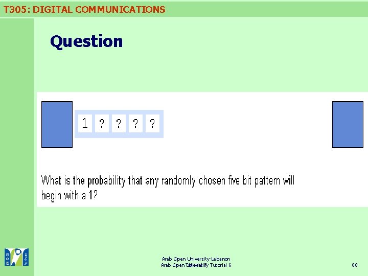
T 305: DIGITAL COMMUNICATIONS Question Arab Open University-Lebanon Arab Open Tutorial University 7 Tutorial 6 88

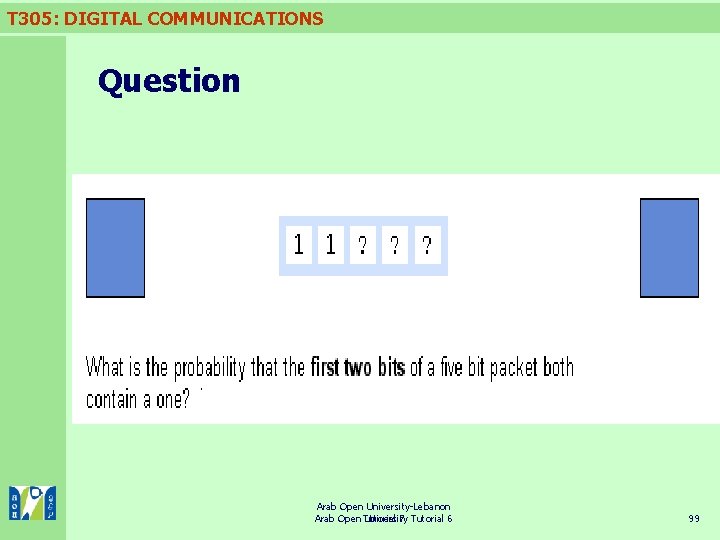
T 305: DIGITAL COMMUNICATIONS Question Arab Open University-Lebanon Arab Open Tutorial University 7 Tutorial 6 99

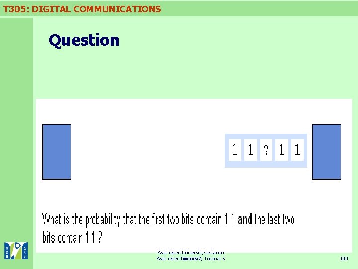
T 305: DIGITAL COMMUNICATIONS Question Arab Open University-Lebanon Arab Open Tutorial University 7 Tutorial 6 1010

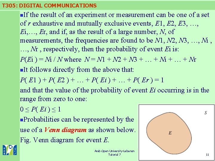
T 305: DIGITAL COMMUNICATIONS If the result of an experiment or measurement can be one of a set of r exhaustive and mutually exclusive events, E 1, E 2, E 3, …, Ei, …, Er, and if, as the result of a large number, N, of measurements, the frequencies are found to be N 1, N 2, N 3, …, Ni , …, Nr , respectively, then the probability of event Ei is: P(Ei ) = Ni / N where N = N 1 + N 2 + N 3 + … + Ni + … + Nr n. It follows directly from the above that: P( E 1 ) + P( E 2 ) + … + P( Ei ) + … + P( Er ) = 1 and that the value of the probability of event Ei occurring is in the range from zero to one: 0 ≤ P( Ei ) ≤ 1 n. Probabilities can be represented by the use of a Venn diagram as shown below. Fig. Venn diagram for event E. n Arab Open University-Lebanon Tutorial 7 11

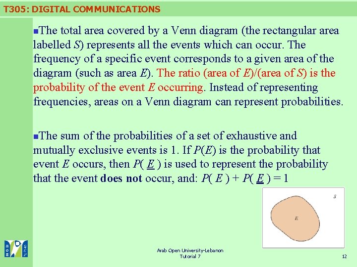
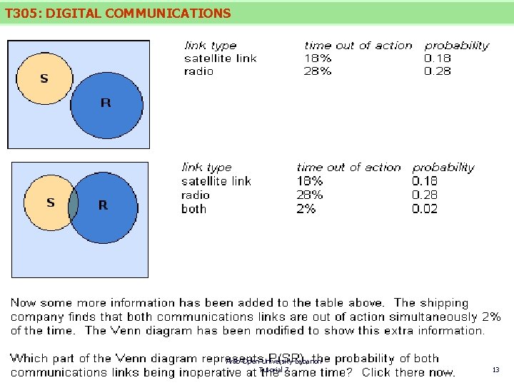
T 305: DIGITAL COMMUNICATIONS The total area covered by a Venn diagram (the rectangular area labelled S) represents all the events which can occur. The frequency of a specific event corresponds to a given area of the diagram (such as area E). The ratio (area of E)/(area of S) is the probability of the event E occurring. Instead of representing frequencies, areas on a Venn diagram can represent probabilities. n The sum of the probabilities of a set of exhaustive and mutually exclusive events is 1. If P(E) is the probability that event E occurs, then P( E ) is used to represent the probability that the event does not occur, and: P( E ) + P( E ) = 1 n Arab Open University-Lebanon Tutorial 7 12

T 305: DIGITAL COMMUNICATIONS Arab Open University-Lebanon Tutorial 7 13

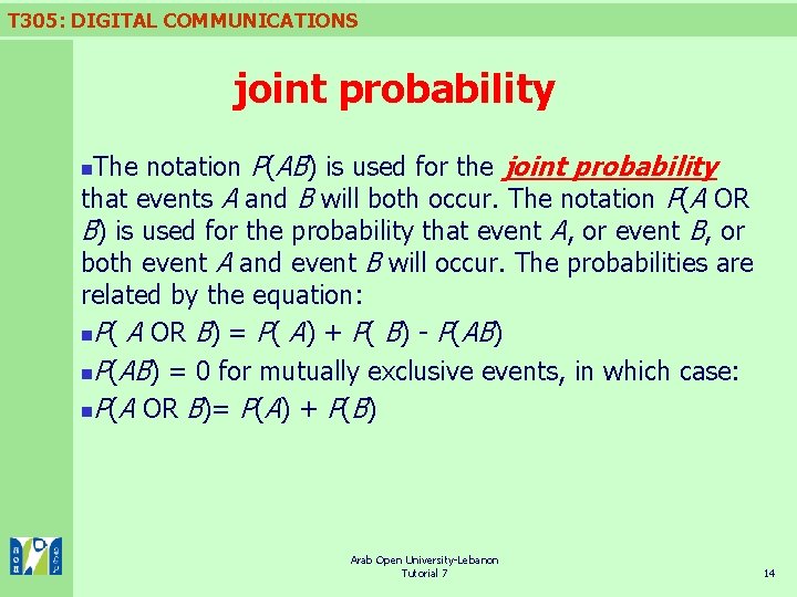
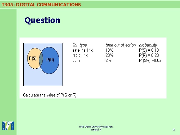
T 305: DIGITAL COMMUNICATIONS joint probability The notation P(AB) is used for the joint probability that events A and B will both occur. The notation P(A OR B) is used for the probability that event A, or event B, or both event A and event B will occur. The probabilities are related by the equation: n. P( A OR B) = P( A) + P( B) - P(AB) n. P(AB) = 0 for mutually exclusive events, in which case: n. P(A OR B)= P(A) + P(B) n Arab Open University-Lebanon Tutorial 7 14

T 305: DIGITAL COMMUNICATIONS Question Arab Open University-Lebanon Tutorial 7 15

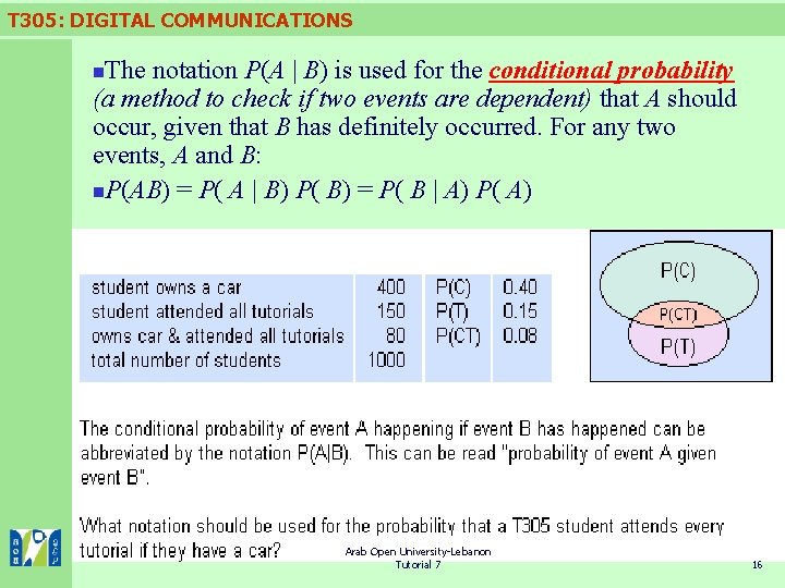
T 305: DIGITAL COMMUNICATIONS The notation P(A | B) is used for the conditional probability (a method to check if two events are dependent) that A should occur, given that B has definitely occurred. For any two events, A and B: n. P(AB) = P( A | B) P( B) = P( B | A) P( A) n Arab Open University-Lebanon Tutorial 7 16

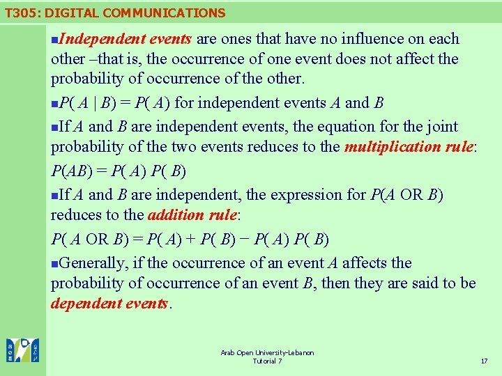
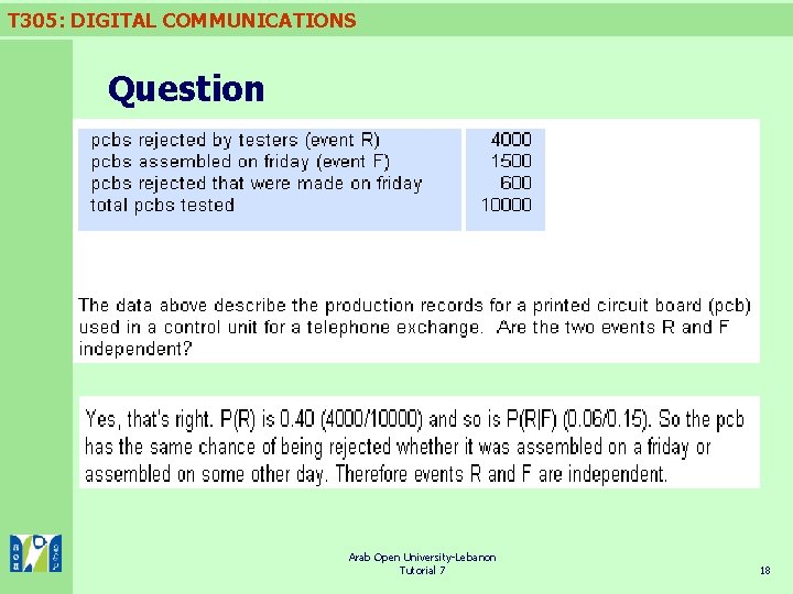
T 305: DIGITAL COMMUNICATIONS Independent events are ones that have no influence on each other –that is, the occurrence of one event does not affect the probability of occurrence of the other. n. P( A | B) = P( A) for independent events A and B n. If A and B are independent events, the equation for the joint probability of the two events reduces to the multiplication rule: P(AB) = P( A) P( B) n. If A and B are independent, the expression for P(A OR B) reduces to the addition rule: P( A OR B) = P( A) + P( B) − P( A) P( B) n. Generally, if the occurrence of an event A affects the probability of occurrence of an event B, then they are said to be dependent events. n Arab Open University-Lebanon Tutorial 7 17

T 305: DIGITAL COMMUNICATIONS Question Arab Open University-Lebanon Tutorial 7 18

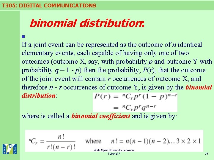
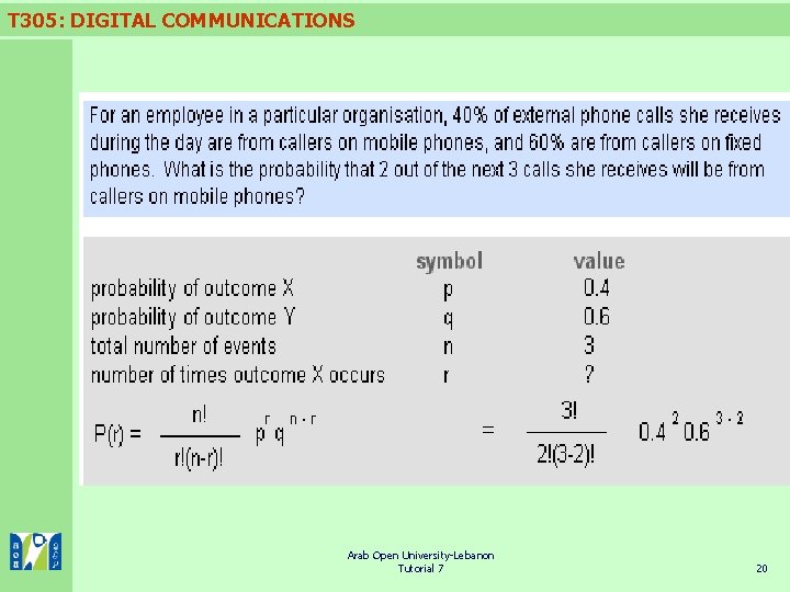
T 305: DIGITAL COMMUNICATIONS binomial distribution: n If a joint event can be represented as the outcome of n identical elementary events, each capable of having only one of two outcomes (outcome X, say, with probability p and outcome Y with probability q = 1 - p) then the probability, P(r), that the outcome of the joint event will contain r occurrences of outcome X, and therefore n - r occurrences of outcome Y, is given by the binomial distribution: where is called a binomial coefficient and is given by: Arab Open University-Lebanon Tutorial 7 19

T 305: DIGITAL COMMUNICATIONS Arab Open University-Lebanon Tutorial 7 20

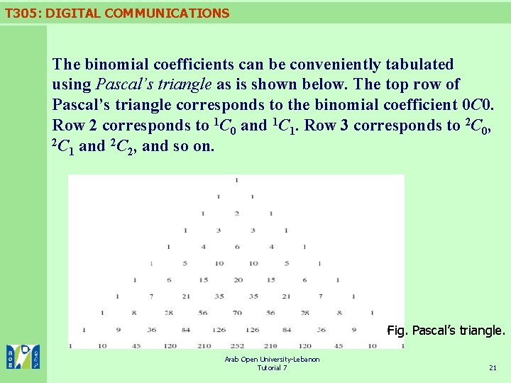
T 305: DIGITAL COMMUNICATIONS The binomial coefficients can be conveniently tabulated using Pascal’s triangle as is shown below. The top row of Pascal’s triangle corresponds to the binomial coefficient 0 C 0. Row 2 corresponds to 1 C 0 and 1 C 1. Row 3 corresponds to 2 C 0, 2 C and 2 C , and so on. 1 2 Fig. Pascal’s triangle. Arab Open University-Lebanon Tutorial 7 21

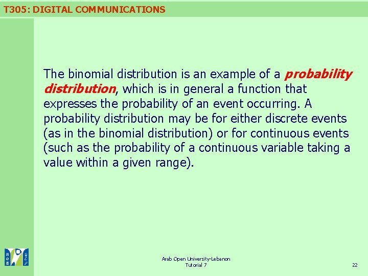
T 305: DIGITAL COMMUNICATIONS The binomial distribution is an example of a probability distribution, which is in general a function that expresses the probability of an event occurring. A probability distribution may be for either discrete events (as in the binomial distribution) or for continuous events (such as the probability of a continuous variable taking a value within a given range). Arab Open University-Lebanon Tutorial 7 22

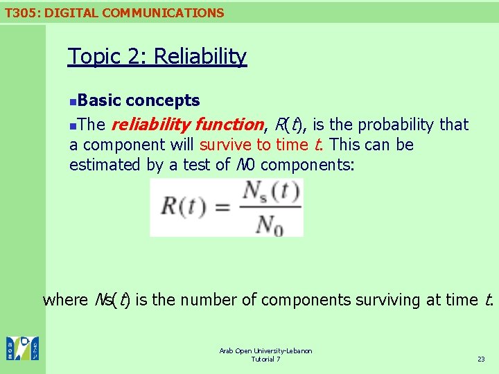
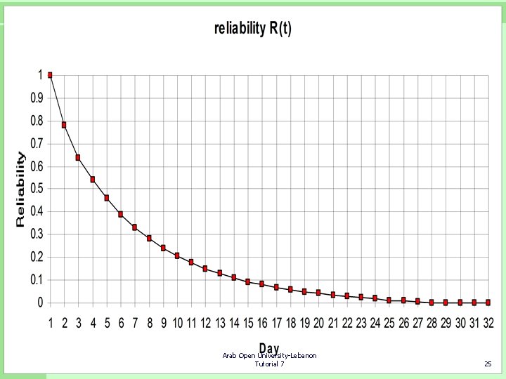
T 305: DIGITAL COMMUNICATIONS Topic 2: Reliability Basic concepts n. The reliability function, R(t), is the probability that a component will survive to time t. This can be estimated by a test of N 0 components: n where Ns(t) is the number of components surviving at time t. Arab Open University-Lebanon Tutorial 7 23

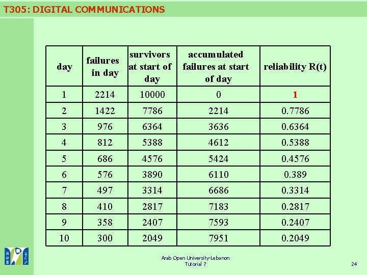
T 305: DIGITAL COMMUNICATIONS day survivors failures at start of in day accumulated failures at start of day reliability R(t) 1 2214 10000 0 1 2 1422 7786 2214 0. 7786 3 976 6364 3636 0. 6364 4 812 5388 4612 0. 5388 5 686 4576 5424 0. 4576 6 576 3890 6110 0. 389 7 497 3314 6686 0. 3314 8 410 2817 7183 0. 2817 9 358 2407 7593 0. 2407 10 300 2049 7951 0. 2049 Arab Open University-Lebanon Tutorial 7 24

T 305: DIGITAL COMMUNICATIONS Arab Open University-Lebanon Tutorial 7 25

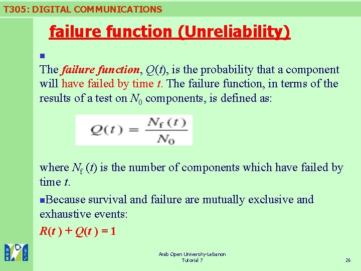
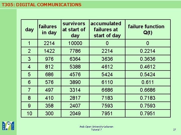
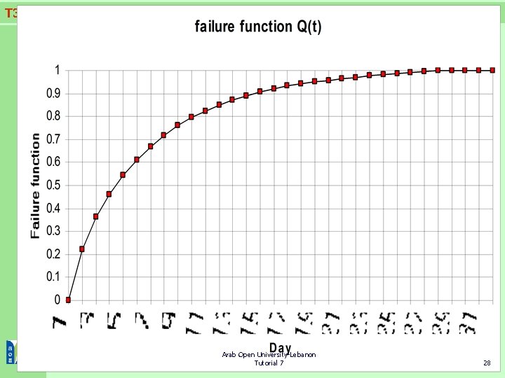
T 305: DIGITAL COMMUNICATIONS failure function (Unreliability) n The failure function, Q(t), is the probability that a component will have failed by time t. The failure function, in terms of the results of a test on N 0 components, is defined as: where Nf (t) is the number of components which have failed by time t. n. Because survival and failure are mutually exclusive and exhaustive events: R(t ) + Q(t ) = 1 Arab Open University-Lebanon Tutorial 7 26

T 305: DIGITAL COMMUNICATIONS day failures in day survivors at start of day accumulated failures at start of day failure function Q(t) 1 2214 10000 0 0 2 1422 7786 2214 0. 2214 3 976 6364 3636 0. 3636 4 812 5388 4612 0. 4612 5 686 4576 5424 0. 5424 6 576 3890 6110 0. 611 7 497 3314 6686 0. 6686 8 410 2817 7183 0. 7183 9 358 2407 7593 0. 7593 10 300 2049 7951 0. 7951 Arab Open University-Lebanon Tutorial 7 27

T 305: DIGITAL COMMUNICATIONS Arab Open University-Lebanon Tutorial 7 28

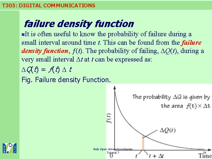
T 305: DIGITAL COMMUNICATIONS failure density function It is often useful to know the probability of failure during a small interval around time t. This can be found from the failure density function, ƒ(t). The probability of failing, Q(t), during a very small interval t at t can be expressed as: Q( t) = ƒ ( t) t Fig. Failure density Function. n Arab Open University-Lebanon Tutorial 7 29

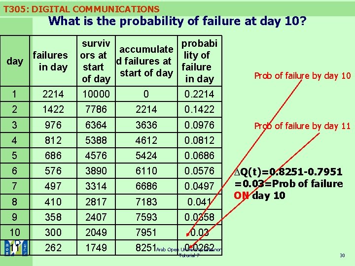
T 305: DIGITAL COMMUNICATIONS What is the probability of failure at day 10? day failures in day surviv probabi accumulate ors at lity of d failures at start failure start of day in day 1 2214 10000 0 0. 2214 2 1422 7786 2214 0. 1422 3 976 6364 3636 0. 0976 4 812 5388 4612 0. 0812 5 686 4576 5424 0. 0686 6 576 3890 6110 0. 0576 7 497 3314 6686 0. 0497 8 410 2817 7183 0. 041 9 358 2407 7593 0. 0358 10 300 2049 7951 0. 03 11 262 1749 8251 Arab Open University-Lebanon 0. 0262 Tutorial 7 Prob of failure by day 10 Prob of failure by day 11 Q(t)=0. 8251 -0. 7951 =0. 03=Prob of failure ON day 10 30

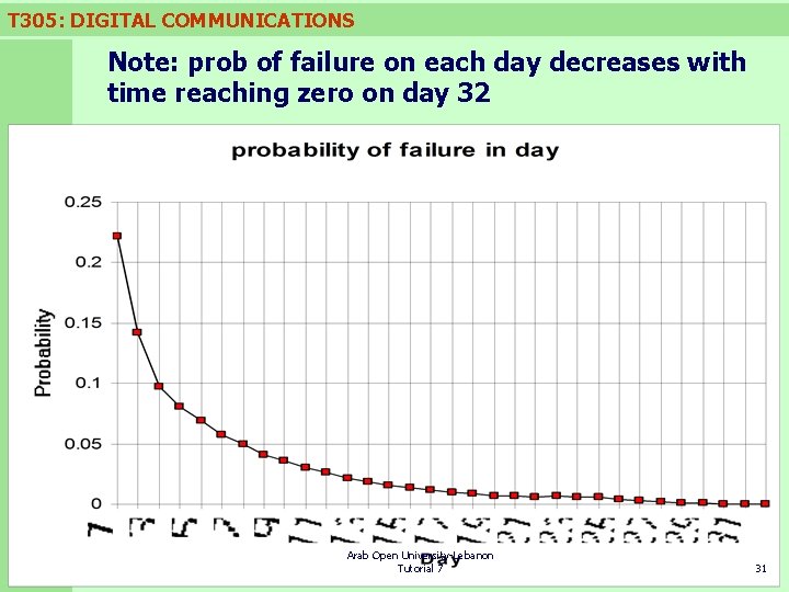
T 305: DIGITAL COMMUNICATIONS Note: prob of failure on each day decreases with time reaching zero on day 32 Arab Open University-Lebanon Tutorial 7 31

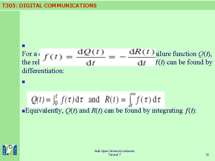
T 305: DIGITAL COMMUNICATIONS n For a continuous reliability function R(t) and failure function Q(t), the relationship to the failure density function ƒ(t) can be found by differentiation: n n Equivalently, Q(t) and R(t) can be found by integrating ƒ(t): Arab Open University-Lebanon Tutorial 7 32

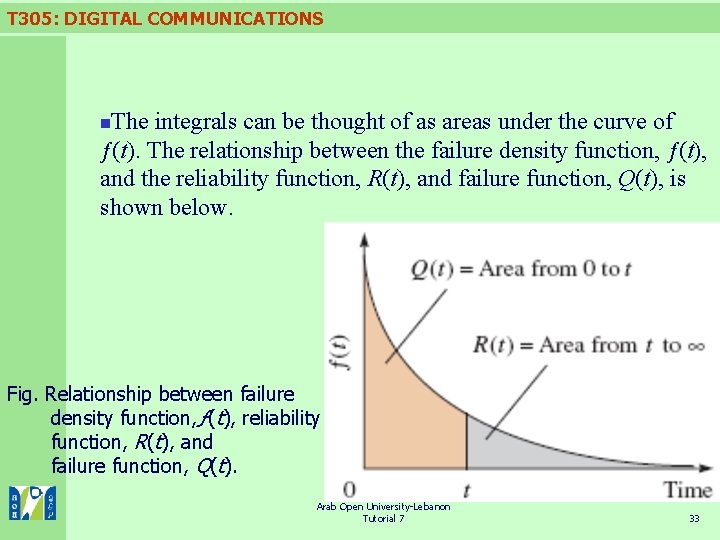
T 305: DIGITAL COMMUNICATIONS The integrals can be thought of as areas under the curve of ƒ(t). The relationship between the failure density function, ƒ(t), and the reliability function, R(t), and failure function, Q(t), is shown below. n Fig. Relationship between failure density function, ƒ(t), reliability function, R(t), and failure function, Q(t). Arab Open University-Lebanon Tutorial 7 33

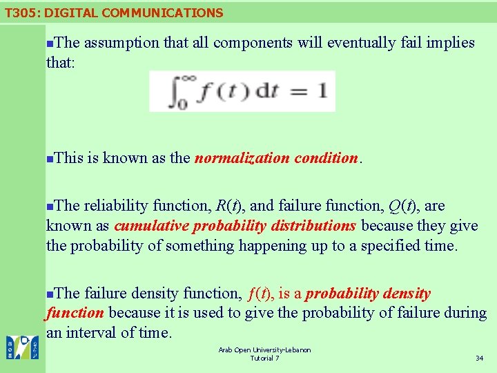
T 305: DIGITAL COMMUNICATIONS The assumption that all components will eventually fail implies that: n n This is known as the normalization condition. The reliability function, R(t), and failure function, Q(t), are known as cumulative probability distributions because they give the probability of something happening up to a specified time. n The failure density function, ƒ(t), is a probability density function because it is used to give the probability of failure during an interval of time. n Arab Open University-Lebanon Tutorial 7 34

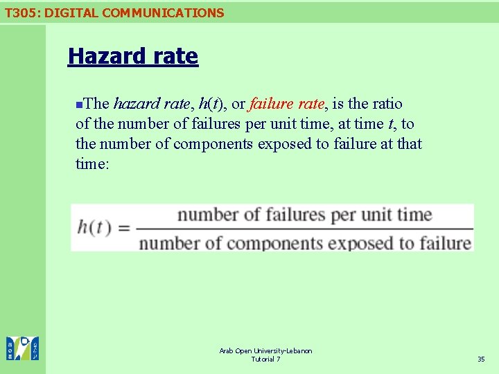
T 305: DIGITAL COMMUNICATIONS Hazard rate The hazard rate, h(t), or failure rate, is the ratio of the number of failures per unit time, at time t, to the number of components exposed to failure at that time: n Arab Open University-Lebanon Tutorial 7 35

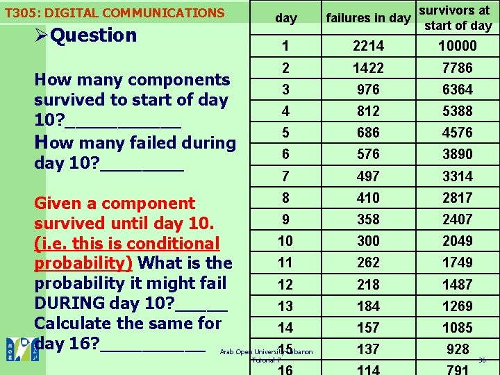
T 305: DIGITAL COMMUNICATIONS ØQuestion day failures in day survivors at start of day 1 2214 10000 2 1422 7786 3 976 6364 4 812 5388 5 686 4576 6 576 3890 7 497 3314 410 2817 358 2407 300 2049 262 1749 218 1487 184 1269 157 1085 137 928 How many components survived to start of day 10? ______ How many failed during day 10? ____ 8 Given a component 9 survived until day 10. 10 (i. e. this is conditional 11 probability) What is the probability it might fail 12 DURING day 10? _____ 13 Calculate the same for 14 day 16? _____ Arab Open University-Lebanon 15 Tutorial 7 36

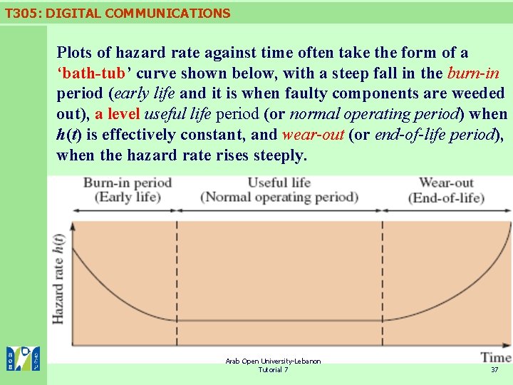
T 305: DIGITAL COMMUNICATIONS Plots of hazard rate against time often take the form of a ‘bath-tub’ curve shown below, with a steep fall in the burn-in period (early life and it is when faulty components are weeded out), a level useful life period (or normal operating period) when h(t) is effectively constant, and wear-out (or end-of-life period), when the hazard rate rises steeply. Arab Open University-Lebanon Tutorial 7 37

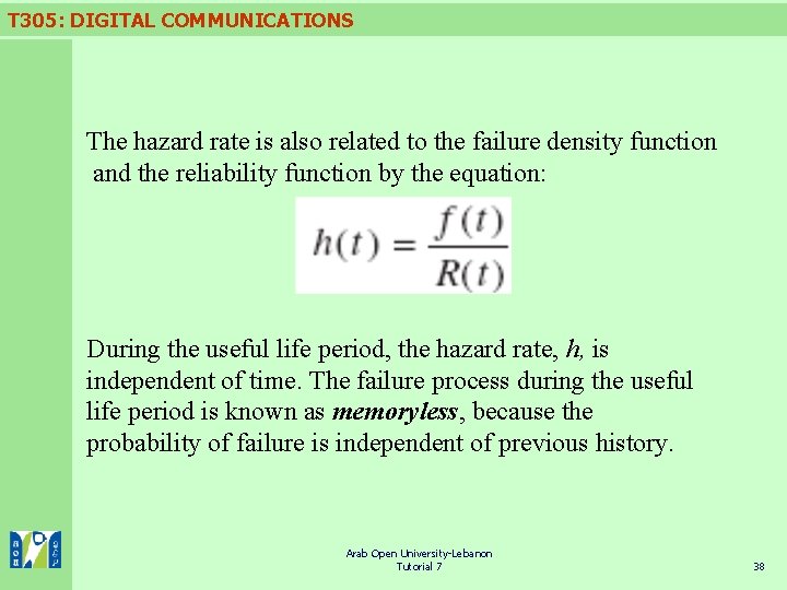
T 305: DIGITAL COMMUNICATIONS The hazard rate is also related to the failure density function and the reliability function by the equation: During the useful life period, the hazard rate, h, is independent of time. The failure process during the useful life period is known as memoryless, because the probability of failure is independent of previous history. Arab Open University-Lebanon Tutorial 7 38

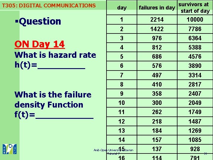
T 305: DIGITAL COMMUNICATIONS §Question ON Day 14 What is hazard rate h(t)=_____ What is the failure density Function f(t)=______ day failures in day survivors at start of day 1 2214 10000 2 1422 7786 3 976 6364 4 812 5388 5 686 4576 6 576 3890 7 497 3314 8 410 2817 9 358 2407 10 300 2049 11 262 1749 12 218 1487 13 184 1269 14 157 1085 15 137 928 Arab Open University-Lebanon Tutorial 7 39

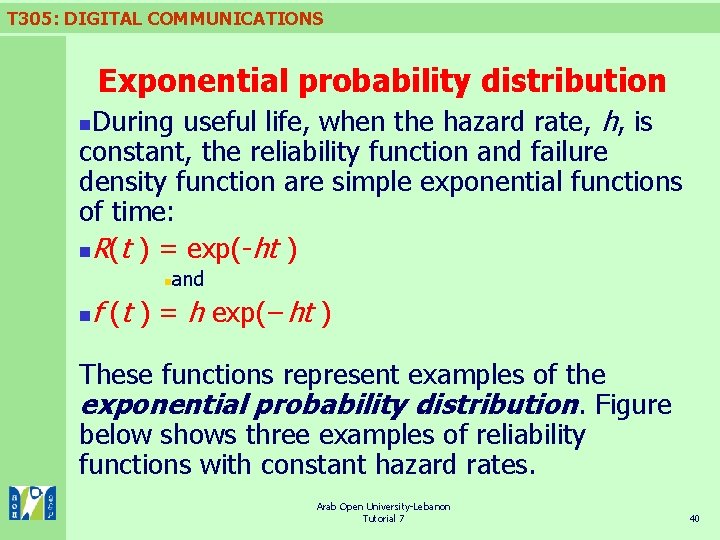
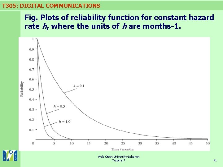
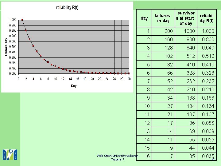
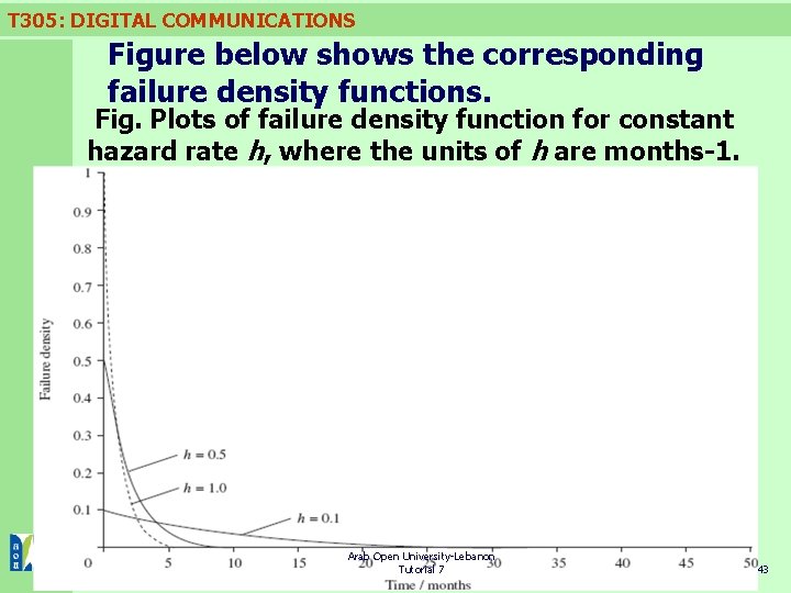
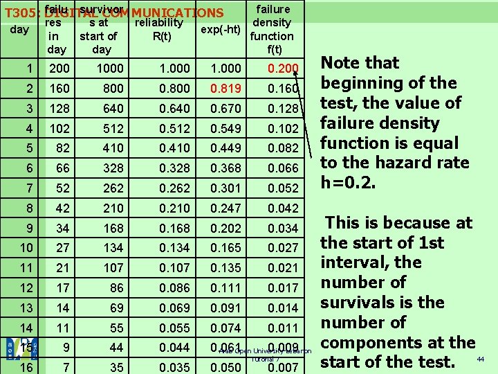
T 305: DIGITAL COMMUNICATIONS Exponential probability distribution During useful life, when the hazard rate, h, is constant, the reliability function and failure density function are simple exponential functions of time: n. R(t ) = exp(-ht ) n n n and f (t ) = h exp(−ht ) These functions represent examples of the exponential probability distribution. Figure below shows three examples of reliability functions with constant hazard rates. Arab Open University-Lebanon Tutorial 7 40

T 305: DIGITAL COMMUNICATIONS Fig. Plots of reliability function for constant hazard rate h, where the units of h are months-1. Arab Open University-Lebanon Tutorial 7 41

T 305: DIGITAL COMMUNICATIONS day Arab Open University-Lebanon Tutorial 7 failures in day survivor s at start of day reliabil ity R(t) 1 200 1000 1. 000 2 160 800 0. 800 3 128 640 0. 640 4 102 512 0. 512 5 82 410 0. 410 6 66 328 0. 328 7 52 262 0. 262 8 42 210 0. 210 9 34 168 0. 168 10 27 134 0. 134 11 21 107 0. 107 12 17 86 0. 086 13 14 69 0. 069 14 11 55 0. 055 15 9 44 0. 044 16 7 35 0. 035 42

T 305: DIGITAL COMMUNICATIONS Figure below shows the corresponding failure density functions. Fig. Plots of failure density function for constant hazard rate h, where the units of h are months-1. Arab Open University-Lebanon Tutorial 7 43

failu survivor T 305: DIGITAL COMMUNICATIONS day res in day s at start of day reliability R(t) failure density exp(-ht) function f(t) 1 200 1000 1. 000 0. 200 2 160 800 0. 819 0. 160 3 128 640 0. 670 0. 128 4 102 512 0. 549 0. 102 5 82 410 0. 449 0. 082 6 66 328 0. 368 0. 066 7 52 262 0. 301 0. 052 8 42 210 0. 247 0. 042 9 34 168 0. 202 0. 034 10 27 134 0. 165 0. 027 11 21 107 0. 135 0. 021 12 17 86 0. 086 0. 111 0. 017 13 14 69 0. 091 0. 014 14 11 55 0. 074 0. 011 15 9 44 0. 061 0. 009 Arab Open University-Lebanon 16 7 35 0. 050 Tutorial 7 0. 007 Note that beginning of the test, the value of failure density function is equal to the hazard rate h=0. 2. This is because at the start of 1 st interval, the number of survivals is the number of components at the start of the test. 44

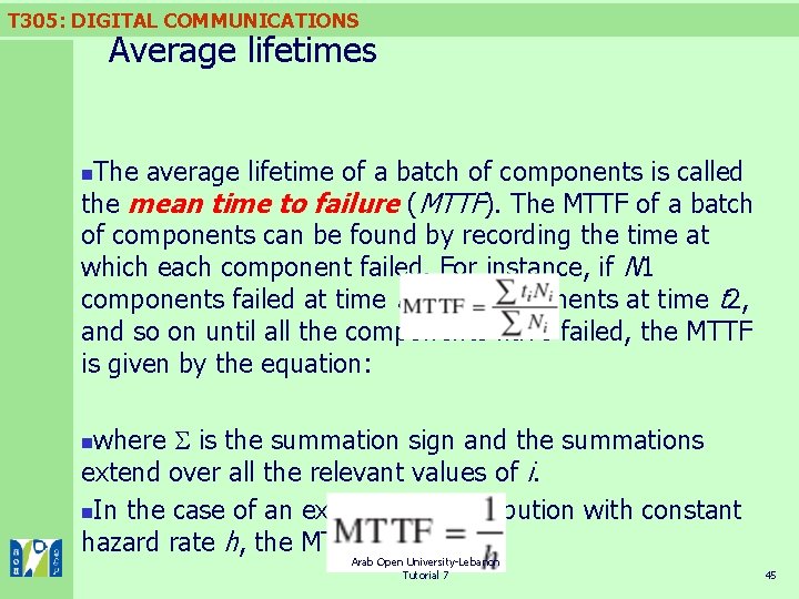
T 305: DIGITAL COMMUNICATIONS Average lifetimes The average lifetime of a batch of components is called the mean time to failure (MTTF). The MTTF of a batch of components can be found by recording the time at which each component failed. For instance, if N 1 components failed at time t 1, N 2 components at time t 2, and so on until all the components have failed, the MTTF is given by the equation: n where is the summation sign and the summations extend over all the relevant values of i. n. In the case of an exponential distribution with constant hazard rate h, the MTTF is simply: n Arab Open University-Lebanon Tutorial 7 45

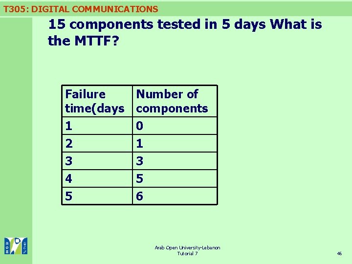
T 305: DIGITAL COMMUNICATIONS 15 components tested in 5 days What is the MTTF? Failure time(days Number of components 1 2 3 4 5 0 1 3 5 6 Arab Open University-Lebanon Tutorial 7 46

T 305: DIGITAL COMMUNICATIONS Confidence levels The degree to which an MTTF estimate for a type of component can be trusted depends on the number of components used in obtaining it. This degree of trust is often expressed in terms of confidence levels. n Arab Open University-Lebanon Tutorial 7 47

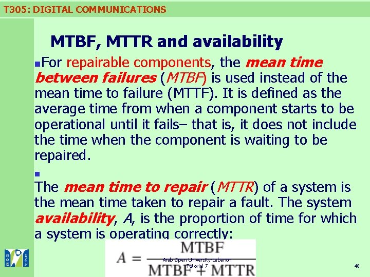
T 305: DIGITAL COMMUNICATIONS MTBF, MTTR and availability For repairable components, the mean time between failures (MTBF) is used instead of the mean time to failure (MTTF). It is defined as the average time from when a component starts to be operational until it fails– that is, it does not include the time when the component is waiting to be repaired. n n The mean time to repair (MTTR) of a system is the mean time taken to repair a fault. The system availability, A, is the proportion of time for which a system is operating correctly: Arab Open University-Lebanon Tutorial 7 48

T 305: DIGITAL COMMUNICATIONS Topic 3: Preparation for Next Tutorial Please inform the students to do the following activities before coming to the next tutorial: n. Overview the Contents of Block n Arab Open University-Lebanon Tutorial 7 49