szeliski 2 1 5 Image Features Computer Vision






- Slides: 83

szeliski 2. 1. 5 Image Features Computer Vision 6. 869 Bill Freeman Image and shape descriptors: Harris corner detectors and SIFT features. With slides from Darya Frolova, Denis Simakov, David Lowe

9

Uses for feature point detectors and descriptors in computer vision and graphics. – – – – Image alignment and building panoramas 3 D reconstruction Motion tracking Object recognition Indexing and database retrieval Robot navigation … other

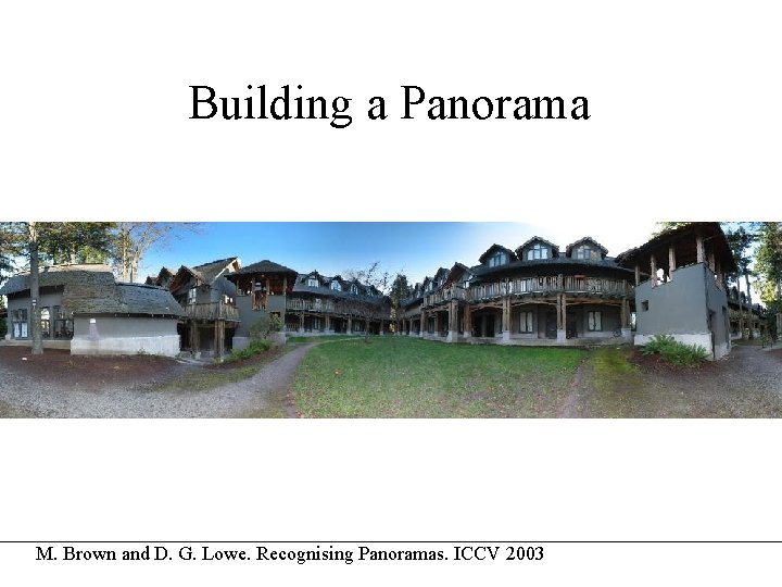
How do we build a panorama? • We need to match (align) images

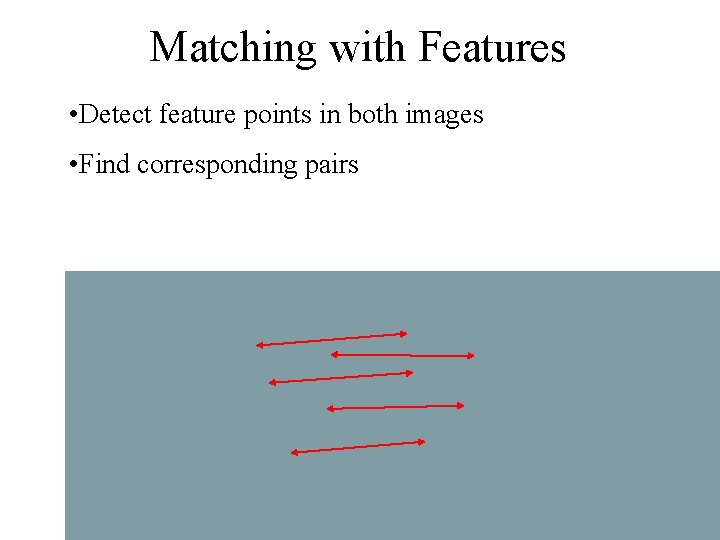
Matching with Features • Detect feature points in both images

Matching with Features • Detect feature points in both images • Find corresponding pairs

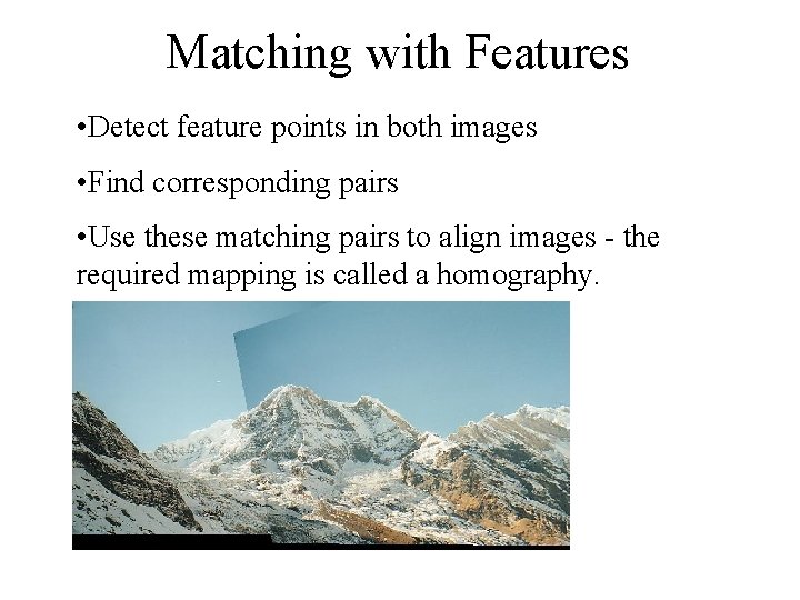
Matching with Features • Detect feature points in both images • Find corresponding pairs • Use these matching pairs to align images - the required mapping is called a homography.

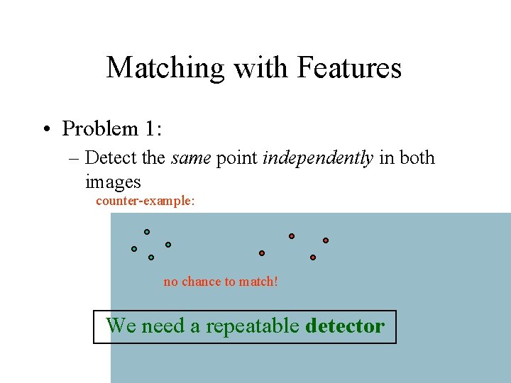
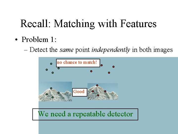
Matching with Features • Problem 1: – Detect the same point independently in both images counter-example: no chance to match! We need a repeatable detector

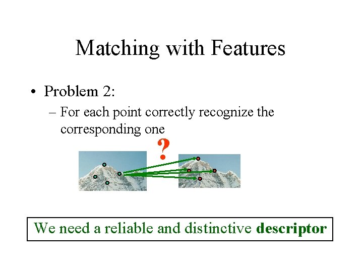
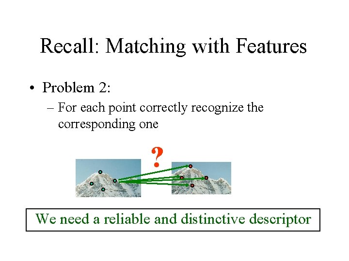
Matching with Features • Problem 2: – For each point correctly recognize the corresponding one ? We need a reliable and distinctive descriptor

Building a Panorama M. Brown and D. G. Lowe. Recognising Panoramas. ICCV 2003

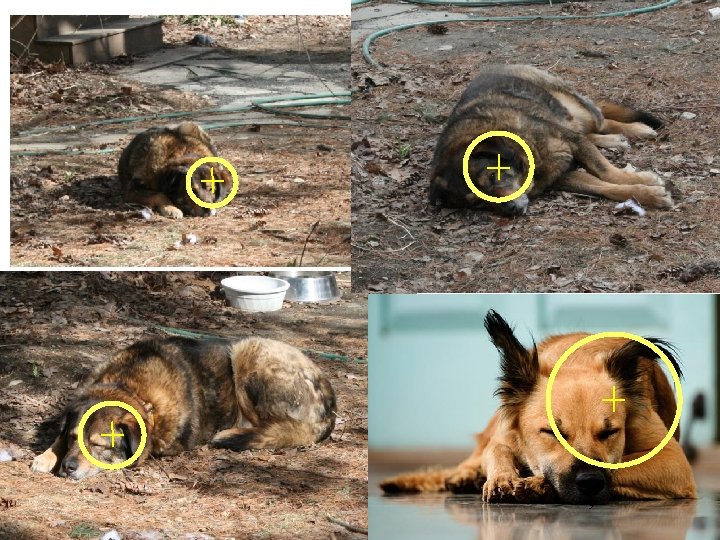
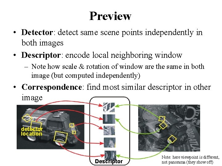
Preview • Detector: detect same scene points independently in both images • Descriptor: encode local neighboring window – Note how scale & rotation of window are the same in both image (but computed independently) • Correspondence: find most similar descriptor in other image detector location Descriptor Note: here viewpoint is different, not panorama (they show off)

Outline • Feature point detection – Harris corner detector – finding a characteristic scale • Local image description – SIFT features 24

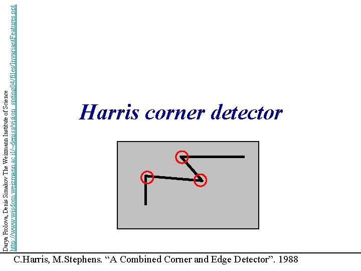
http: //www. wisdom. weizmann. ac. il/~deniss/vision_spring 04/files/Invariant. Features. ppt Darya Frolova, Denis Simakov The Weizmann Institute of Science Harris corner detector C. Harris, M. Stephens. “A Combined Corner and Edge Detector”. 1988

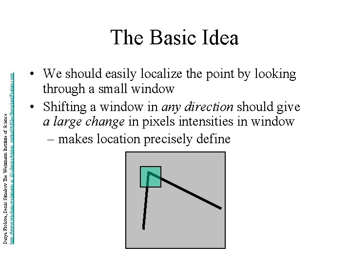
Darya Frolova, Denis Simakov The Weizmann Institute of Science http: //www. wisdom. weizmann. ac. il/~deniss/vision_spring 04/files/Invariant. Features. ppt The Basic Idea • We should easily localize the point by looking through a small window • Shifting a window in any direction should give a large change in pixels intensities in window – makes location precisely define

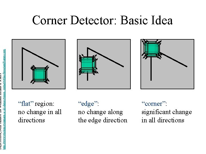
Darya Frolova, Denis Simakov The Weizmann Institute of Science http: //www. wisdom. weizmann. ac. il/~deniss/vision_spring 04/files/Invariant. Features. ppt Corner Detector: Basic Idea “flat” region: no change in all directions “edge”: no change along the edge direction “corner”: significant change in all directions

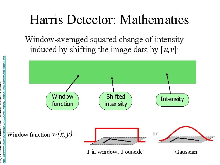
Darya Frolova, Denis Simakov The Weizmann Institute of Science http: //www. wisdom. weizmann. ac. il/~deniss/vision_spring 04/files/Invariant. Features. ppt Harris Detector: Mathematics Window-averaged squared change of intensity induced by shifting the image data by [u, v]: Window function Shifted intensity Window function w(x, y) = Intensity or 1 in window, 0 outside Gaussian

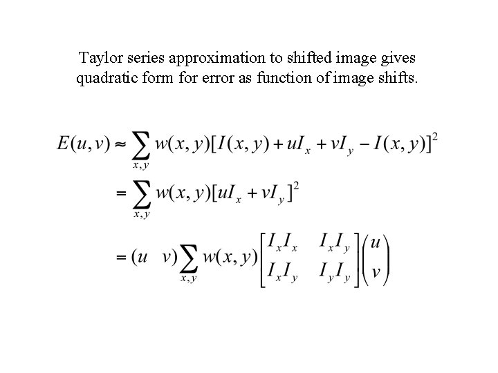
Taylor series approximation to shifted image gives quadratic form for error as function of image shifts.

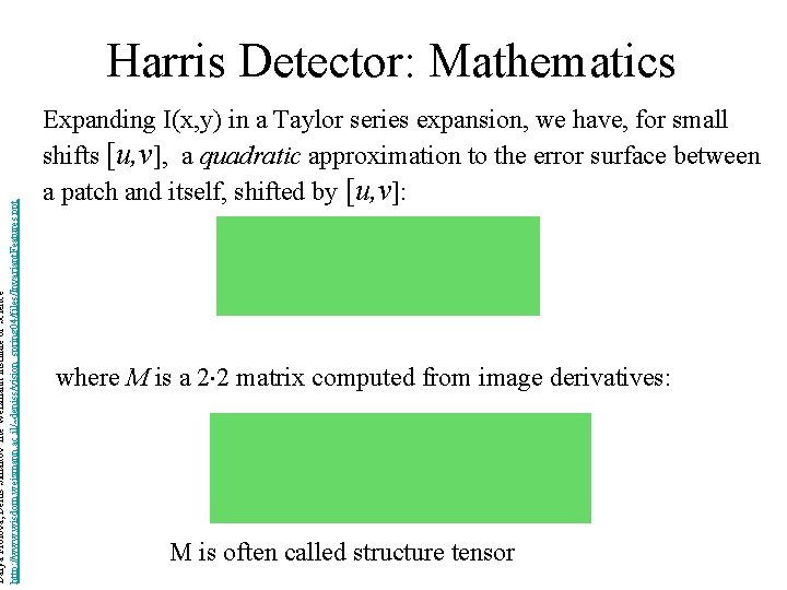
Darya Frolova, Denis Simakov The Weizmann Institute of Science http: //www. wisdom. weizmann. ac. il/~deniss/vision_spring 04/files/Invariant. Features. ppt Harris Detector: Mathematics Expanding I(x, y) in a Taylor series expansion, we have, for small shifts [u, v], a quadratic approximation to the error surface between a patch and itself, shifted by [u, v]: where M is a 2× 2 matrix computed from image derivatives: M is often called structure tensor

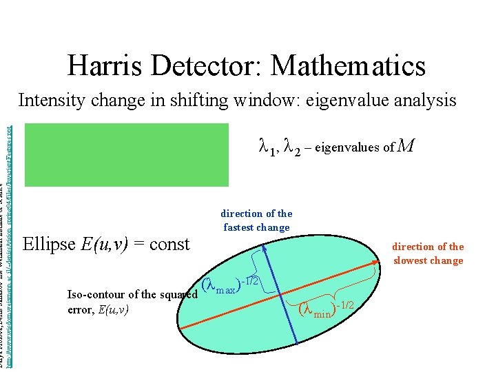
Darya Frolova, Denis Simakov The Weizmann Institute of Science http: //www. wisdom. weizmann. ac. il/~deniss/vision_spring 04/files/Invariant. Features. ppt Harris Detector: Mathematics Intensity change in shifting window: eigenvalue analysis λ 1, λ 2 – eigenvalues of M Ellipse E(u, v) = const Iso-contour of the squared error, E(u, v) direction of the fastest change direction of the slowest change (λ max)-1/2 (λ min)-1/2

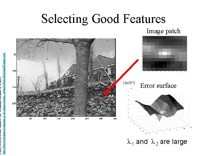
Darya Frolova, Denis Simakov The Weizmann Institute of Science http: //www. wisdom. weizmann. ac. il/~deniss/vision_spring 04/files/Invariant. Features. ppt Selecting Good Features Image patch 12 x 10^5 Error surface λ 1 and λ 2 are large

Darya Frolova, Denis Simakov The Weizmann Institute of Science http: //www. wisdom. weizmann. ac. il/~deniss/vision_spring 04/files/Invariant. Features. ppt Selecting Good Features Image patch 9 x 10^5 Error surface large λ 1, small λ 2

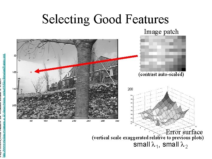
Darya Frolova, Denis Simakov The Weizmann Institute of Science http: //www. wisdom. weizmann. ac. il/~deniss/vision_spring 04/files/Invariant. Features. ppt Selecting Good Features Image patch (contrast auto-scaled) 200 Error surface (vertical scale exaggerated relative to previous plots) small λ 1, small λ 2

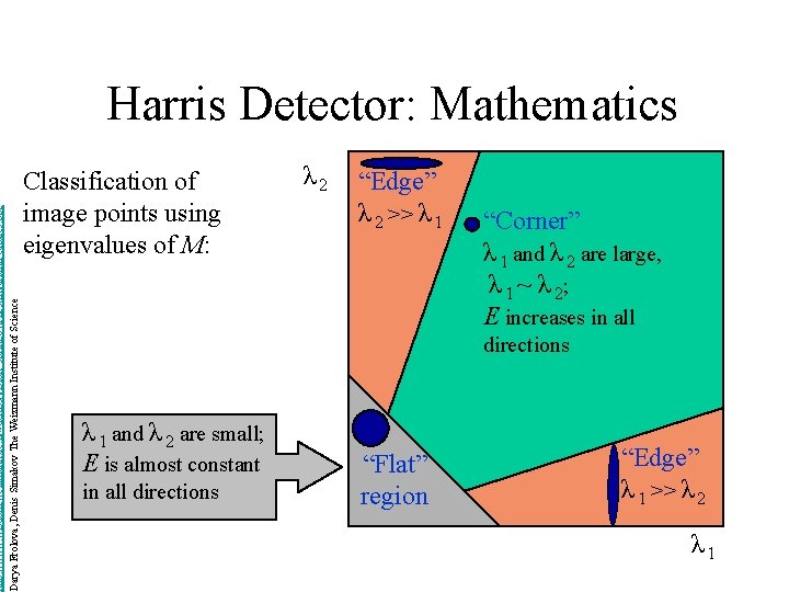
http: //www. wisdom. weizmann. ac. il/~deniss/vision_spring 04/files/Invariant. Features. ppt Darya Frolova, Denis Simakov The Weizmann Institute of Science Harris Detector: Mathematics Classification of image points using eigenvalues of M: λ 2 “Edge” λ 2 >> λ 1 “Corner” λ 1 and λ 2 are large, λ 1 ~ λ 2; E increases in all directions λ 1 and λ 2 are small; E is almost constant in all directions “Flat” region “Edge” λ 1 >> λ 2 λ 1

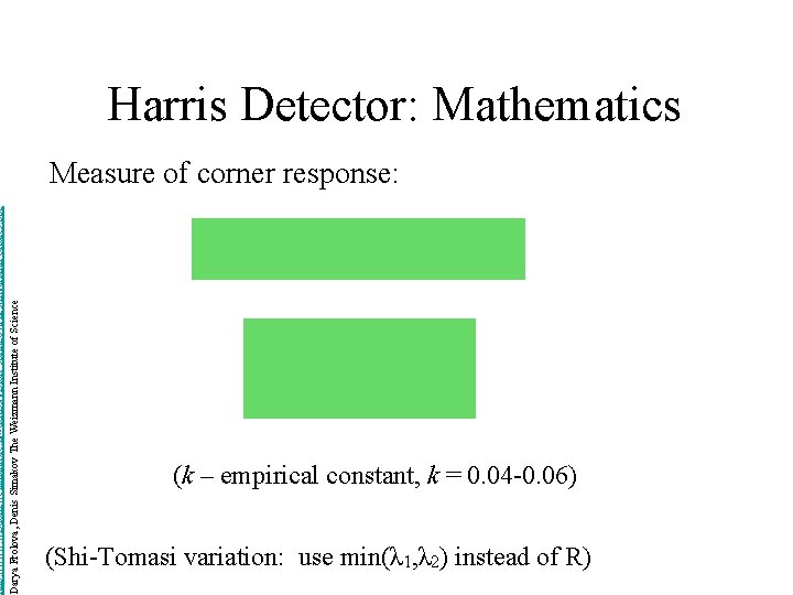
http: //www. wisdom. weizmann. ac. il/~deniss/vision_spring 04/files/Invariant. Features. ppt Darya Frolova, Denis Simakov The Weizmann Institute of Science Harris Detector: Mathematics Measure of corner response: (k – empirical constant, k = 0. 04 -0. 06) (Shi-Tomasi variation: use min(λ 1, λ 2) instead of R)

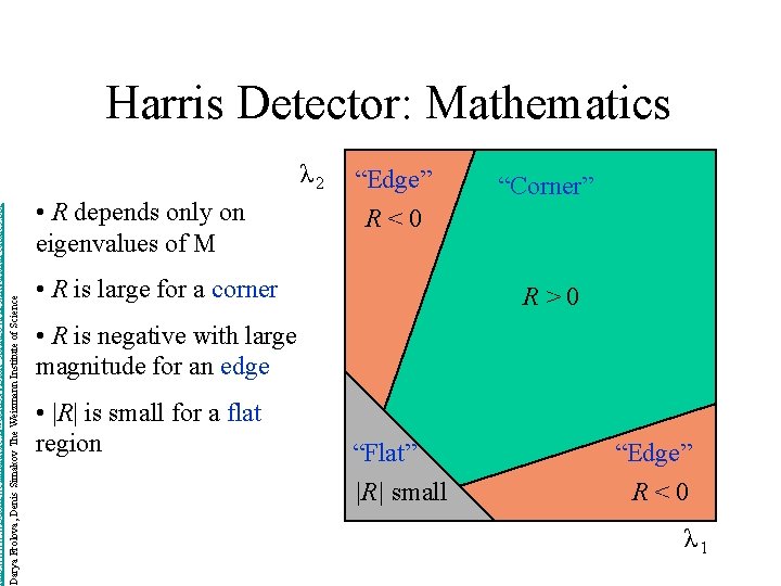
http: //www. wisdom. weizmann. ac. il/~deniss/vision_spring 04/files/Invariant. Features. ppt Darya Frolova, Denis Simakov The Weizmann Institute of Science Harris Detector: Mathematics λ 2 • R depends only on eigenvalues of M “Edge” R<0 • R is large for a corner “Corner” R>0 • R is negative with large magnitude for an edge • |R| is small for a flat region “Flat” |R| small “Edge” R<0 λ 1

Harris Detector • The Algorithm: – Find points with large corner response function R (R > threshold) – Take the points of local maxima of R

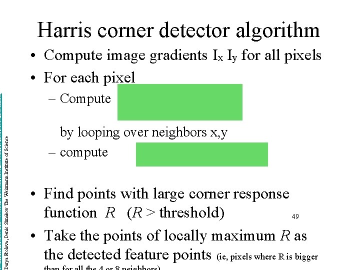
http: //www. wisdom. weizmann. ac. il/~deniss/vision_spring 04/files/Invariant. Features. ppt Darya Frolova, Denis Simakov The Weizmann Institute of Science Harris corner detector algorithm • Compute image gradients Ix Iy for all pixels • For each pixel – Compute by looping over neighbors x, y – compute • Find points with large corner response function R (R > threshold) 49 • Take the points of locally maximum R as the detected feature points (ie, pixels where R is bigger

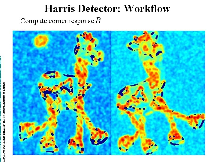
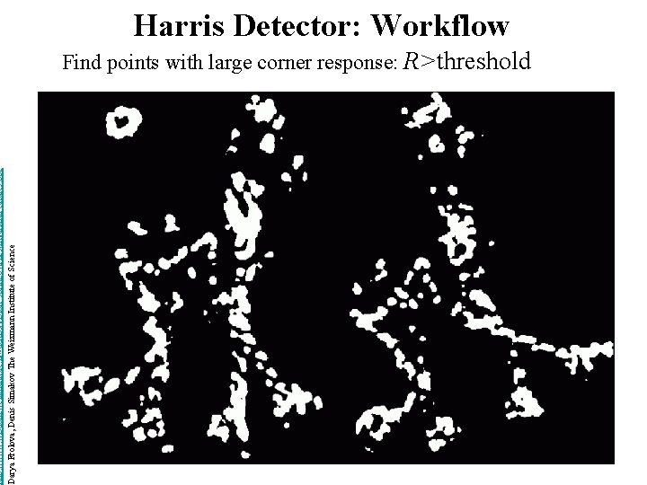
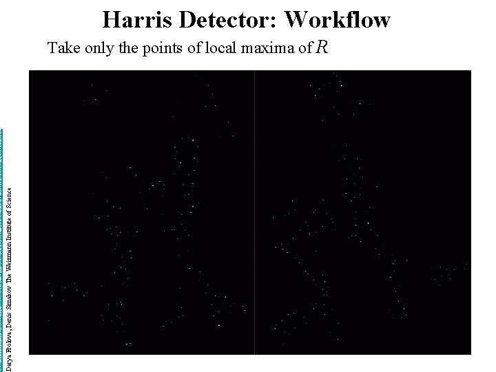
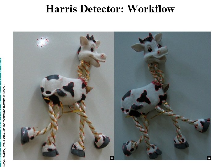
http: //www. wisdom. weizmann. ac. il/~deniss/vision_spring 04/files/Invariant. Features. ppt Darya Frolova, Denis Simakov The Weizmann Institute of Science Harris Detector: Workflow

http: //www. wisdom. weizmann. ac. il/~deniss/vision_spring 04/files/Invariant. Features. ppt Darya Frolova, Denis Simakov The Weizmann Institute of Science Harris Detector: Workflow Compute corner response R

http: //www. wisdom. weizmann. ac. il/~deniss/vision_spring 04/files/Invariant. Features. ppt Darya Frolova, Denis Simakov The Weizmann Institute of Science Harris Detector: Workflow Find points with large corner response: R>threshold

http: //www. wisdom. weizmann. ac. il/~deniss/vision_spring 04/files/Invariant. Features. ppt Darya Frolova, Denis Simakov The Weizmann Institute of Science Harris Detector: Workflow Take only the points of local maxima of R

http: //www. wisdom. weizmann. ac. il/~deniss/vision_spring 04/files/Invariant. Features. ppt Darya Frolova, Denis Simakov The Weizmann Institute of Science Harris Detector: Workflow

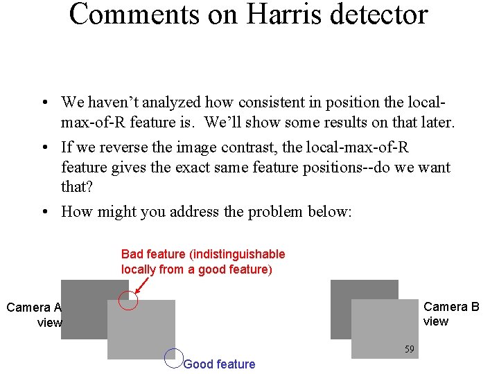
Comments on Harris detector • We haven’t analyzed how consistent in position the localmax-of-R feature is. We’ll show some results on that later. • If we reverse the image contrast, the local-max-of-R feature gives the exact same feature positions--do we want that? • How might you address the problem below: Bad feature (indistinguishable locally from a good feature) Camera B view Camera A view 59 Good feature

Analysis of Harris corner detector invariance properties • Geometry – rotation – scale • Photometry – intensity change 60

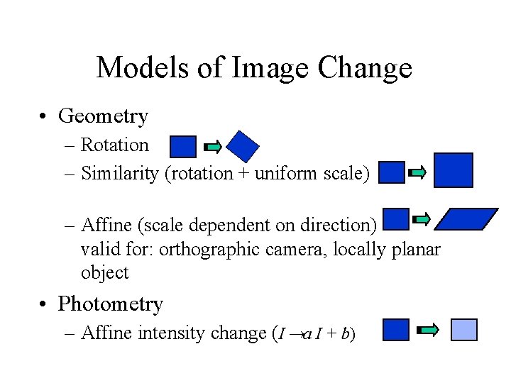
Models of Image Change • Geometry – Rotation – Similarity (rotation + uniform scale) – Affine (scale dependent on direction) valid for: orthographic camera, locally planar object • Photometry – Affine intensity change (I →a I + b)

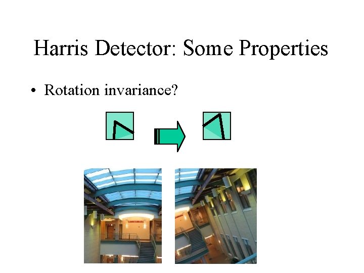
Harris Detector: Some Properties • Rotation invariance?

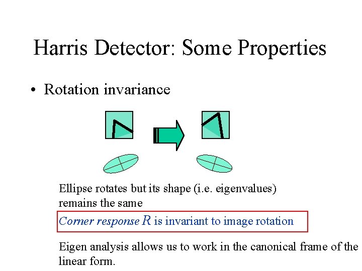
Harris Detector: Some Properties • Rotation invariance Ellipse rotates but its shape (i. e. eigenvalues) remains the same Corner response R is invariant to image rotation Eigen analysis allows us to work in the canonical frame of the linear form.

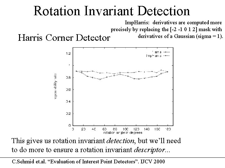
Rotation Invariant Detection Harris Corner Detector Imp. Harris: derivatives are computed more precisely by replacing the [-2 -1 0 1 2] mask with derivatives of a Gaussian (sigma = 1). This gives us rotation invariant detection, but we’ll need to do more to ensure a rotation invariant descriptor. . . C. Schmid et. al. “Evaluation of Interest Point Detectors”. IJCV 2000

Evaluation plots are from this paper

Harris Detector: Some Properties • Invariance to image intensity change?

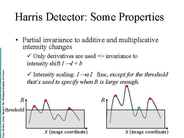
http: //www. wisdom. weizmann. ac. il/~deniss/vision_spring 04/files/Invariant. Features. ppt Darya Frolova, Denis Simakov The Weizmann Institute of Science Harris Detector: Some Properties • Partial invariance to additive and multiplicative intensity changes ü Only derivatives are used => invariance to intensity shift I →I + b ü Intensity scaling: I →a I fine, except for the threshold that’s used to specify when R is large enough. R R threshold x (image coordinate)

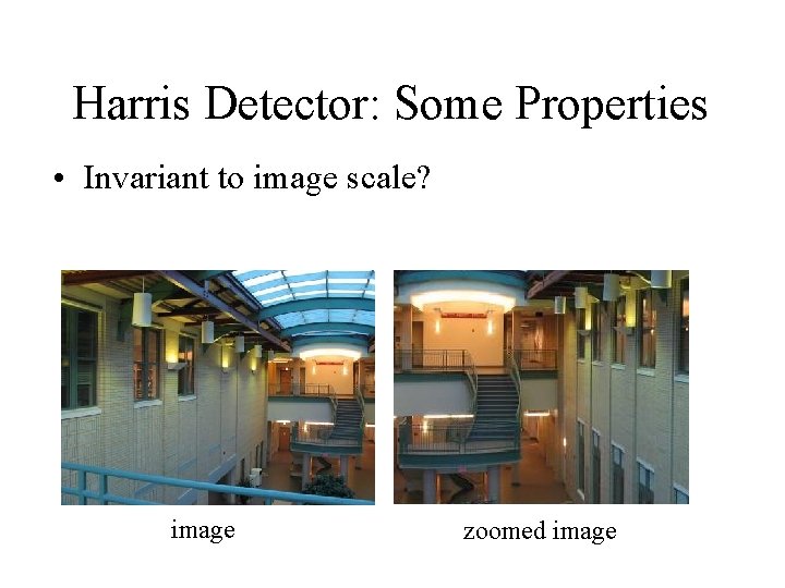
Harris Detector: Some Properties • Invariant to image scale? image zoomed image

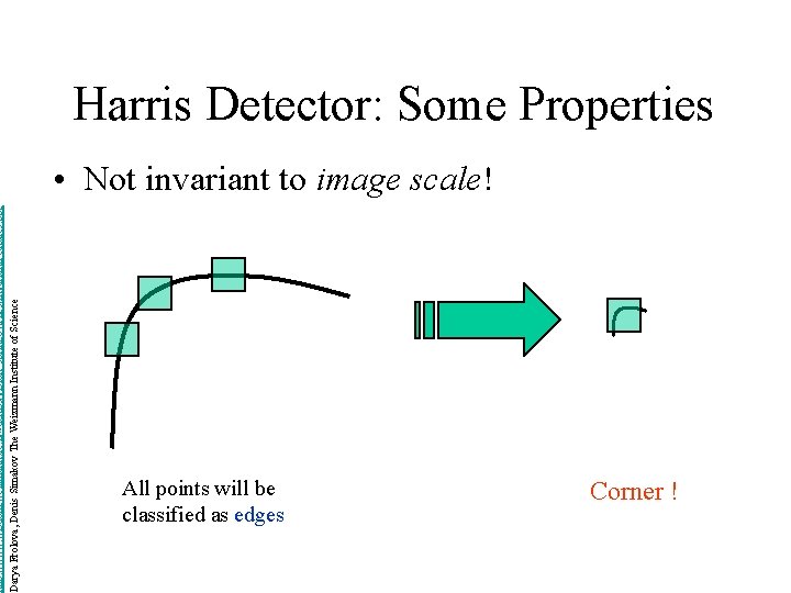
http: //www. wisdom. weizmann. ac. il/~deniss/vision_spring 04/files/Invariant. Features. ppt Darya Frolova, Denis Simakov The Weizmann Institute of Science Harris Detector: Some Properties • Not invariant to image scale! All points will be classified as edges Corner !

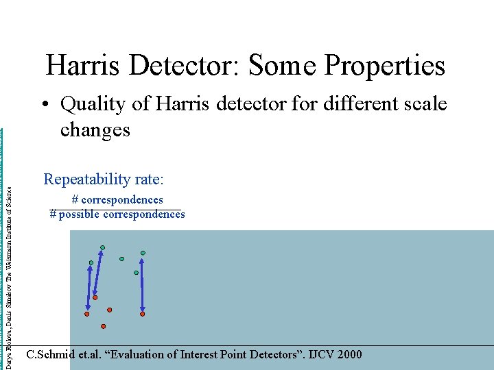
http: //www. wisdom. weizmann. ac. il/~deniss/vision_spring 04/files/Invariant. Features. ppt Darya Frolova, Denis Simakov The Weizmann Institute of Science Harris Detector: Some Properties • Quality of Harris detector for different scale changes Repeatability rate: # correspondences # possible correspondences C. Schmid et. al. “Evaluation of Interest Point Detectors”. IJCV 2000

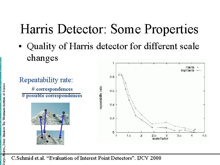
http: //www. wisdom. weizmann. ac. il/~deniss/vision_spring 04/files/Invariant. Features. ppt Darya Frolova, Denis Simakov The Weizmann Institute of Science Harris Detector: Some Properties • Quality of Harris detector for different scale changes Repeatability rate: # correspondences # possible correspondences C. Schmid et. al. “Evaluation of Interest Point Detectors”. IJCV 2000

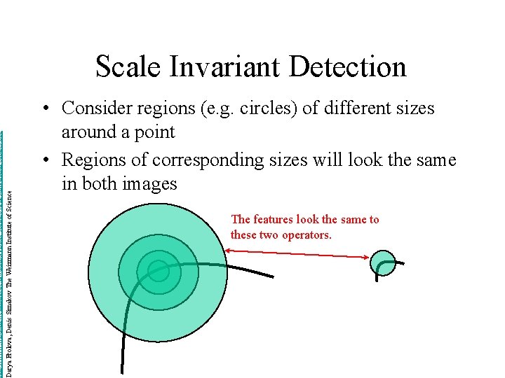
http: //www. wisdom. weizmann. ac. il/~deniss/vision_spring 04/files/Invariant. Features. ppt Darya Frolova, Denis Simakov The Weizmann Institute of Science Scale Invariant Detection • Consider regions (e. g. circles) of different sizes around a point • Regions of corresponding sizes will look the same in both images The features look the same to these two operators.

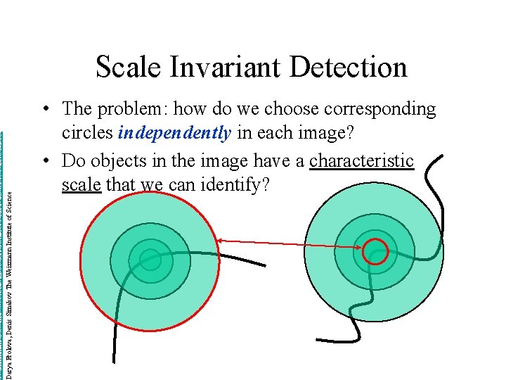
http: //www. wisdom. weizmann. ac. il/~deniss/vision_spring 04/files/Invariant. Features. ppt Darya Frolova, Denis Simakov The Weizmann Institute of Science Scale Invariant Detection • The problem: how do we choose corresponding circles independently in each image? • Do objects in the image have a characteristic scale that we can identify?

Detection over scale Requires a method to repeatably select points in location and scale: • The only reasonable scale-space kernel is a Gaussian (Koenderink, 1984; Lindeberg, 1994) • An efficient choice is to detect peaks in the difference of Gaussian pyramid (Burt & Adelson, 1983; Crowley & Parker, 1984 – but examining more scales) • Difference-of-Gaussian with constant ratio of scales is a close approximation to Lindeberg’s scale-normalized Laplacian (can be shown from the heat diffusion equation)

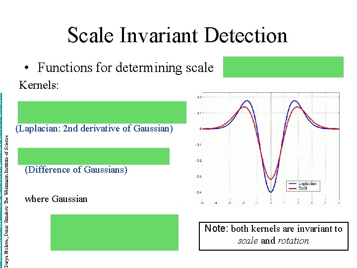
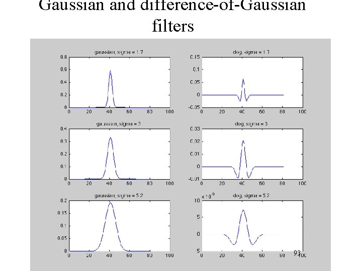
http: //www. wisdom. weizmann. ac. il/~deniss/vision_spring 04/files/Invariant. Features. ppt Darya Frolova, Denis Simakov The Weizmann Institute of Science Scale Invariant Detection • Functions for determining scale Kernels: (Laplacian: 2 nd derivative of Gaussian) (Difference of Gaussians) where Gaussian Note: both kernels are invariant to scale and rotation

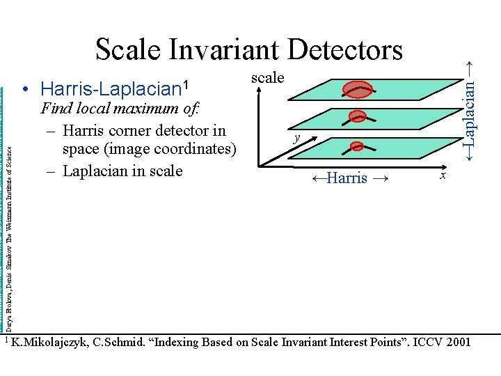
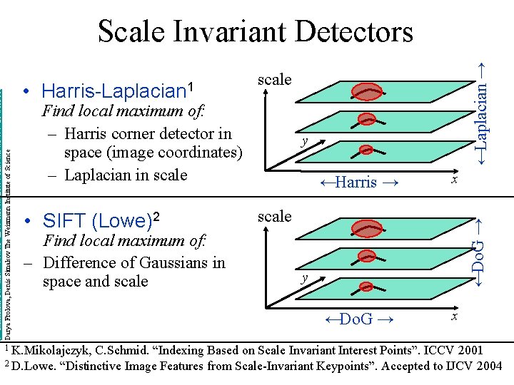
• Harris-Laplacian 1 Find local maximum of: – Harris corner detector in space (image coordinates) – Laplacian in scale 1 K. Mikolajczyk, ←Laplacian → http: //www. wisdom. weizmann. ac. il/~deniss/vision_spring 04/files/Invariant. Features. ppt Darya Frolova, Denis Simakov The Weizmann Institute of Science Scale Invariant Detectors scale y ←Harris → x C. Schmid. “Indexing Based on Scale Invariant Interest Points”. ICCV 2001

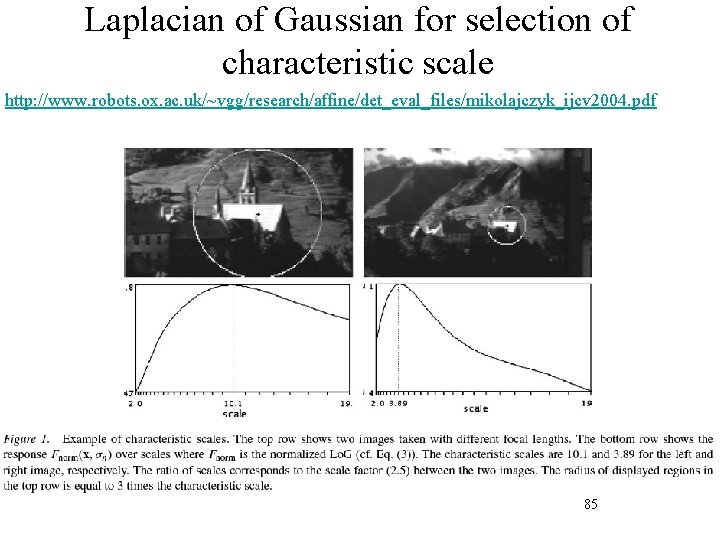
Laplacian of Gaussian for selection of characteristic scale http: //www. robots. ox. ac. uk/~vgg/research/affine/det_eval_files/mikolajczyk_ijcv 2004. pdf 85

scale Find local maximum of: – Harris corner detector in space (image coordinates) – Laplacian in scale • SIFT (Lowe)2 Find local maximum of: – Difference of Gaussians in space and scale 1 K. Mikolajczyk, ←Laplacian → • Harris-Laplacian 1 y ←Harris → x ←Do. G → x scale ←Do. G → http: //www. wisdom. weizmann. ac. il/~deniss/vision_spring 04/files/Invariant. Features. ppt Darya Frolova, Denis Simakov The Weizmann Institute of Science Scale Invariant Detectors y C. Schmid. “Indexing Based on Scale Invariant Interest Points”. ICCV 2001 2 D. Lowe. “Distinctive Image Features from Scale-Invariant Keypoints”. Accepted to IJCV 2004

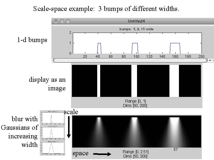
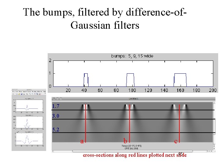
Scale-space example: 3 bumps of different widths. 1 -d bumps display as an image blur with Gaussians of increasing width scale space 87

Gaussian and difference-of-Gaussian filters 93

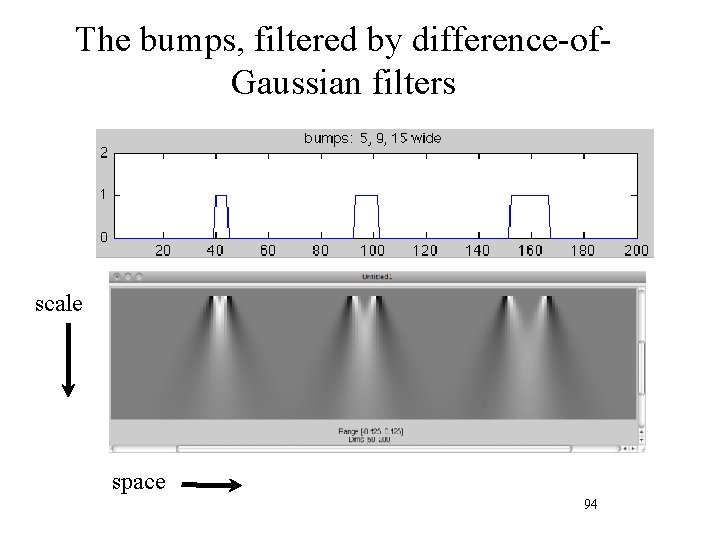
The bumps, filtered by difference-of. Gaussian filters scale space 94

The bumps, filtered by difference-of. Gaussian filters 1. 7 3. 0 5. 2 a b c 95 cross-sections along red lines plotted next slide

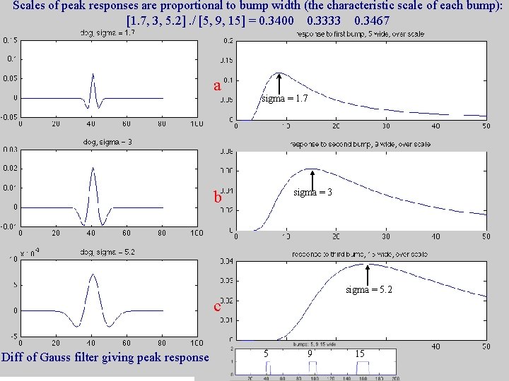
Scales of peak responses are proportional to bump width (the characteristic scale of each bump): [1. 7, 3, 5. 2]. / [5, 9, 15] = 0. 3400 0. 3333 0. 3467 a sigma = 1. 7 sigma = 3 b sigma = 5. 2 c Diff of Gauss filter giving peak response 5 9 15 96

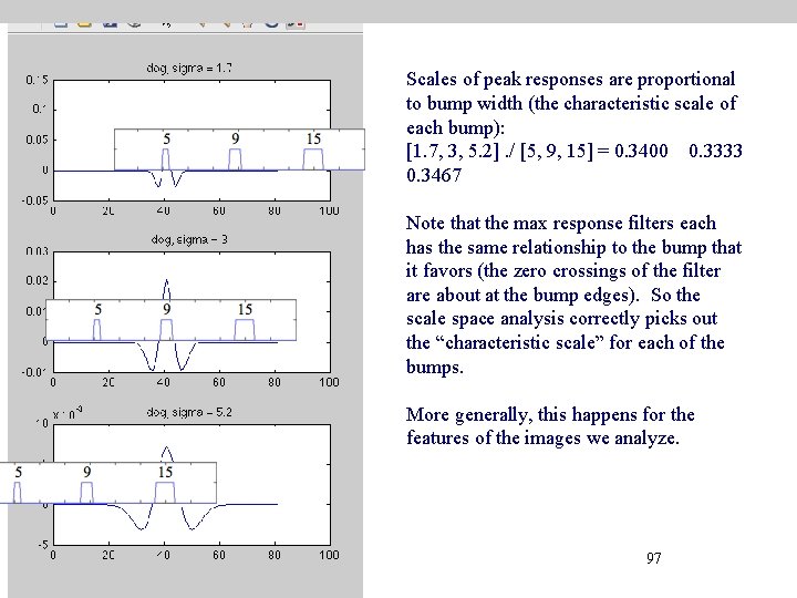
Scales of peak responses are proportional to bump width (the characteristic scale of each bump): [1. 7, 3, 5. 2]. / [5, 9, 15] = 0. 3400 0. 3333 0. 3467 Note that the max response filters each has the same relationship to the bump that it favors (the zero crossings of the filter are about at the bump edges). So the scale space analysis correctly picks out the “characteristic scale” for each of the bumps. More generally, this happens for the features of the images we analyze. 97

Scale Invariant Detectors Darya Frolova, Denis Simakov The Weizmann Institute of Science • Experimental evaluation of detectors w. r. t. scale change Repeatability rate: # correspondences # possible correspondences K. Mikolajczyk, C. Schmid. “Indexing Based on Scale Invariant Interest Points”. ICCV 2001

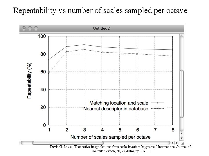
Repeatability vs number of scales sampled per octave David G. Lowe, "Distinctive image features from scale-invariant keypoints, " International Journal of Computer Vision, 60, 2 (2004), pp. 91 -110

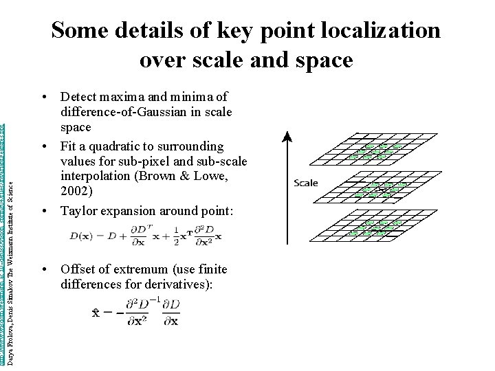
http: //www. wisdom. weizmann. ac. il/~deniss/vision_spring 04/files/Invariant. Features. ppt Darya Frolova, Denis Simakov The Weizmann Institute of Science Some details of key point localization over scale and space • Detect maxima and minima of difference-of-Gaussian in scale space • Fit a quadratic to surrounding values for sub-pixel and sub-scale interpolation (Brown & Lowe, 2002) • Taylor expansion around point: • Offset of extremum (use finite differences for derivatives):

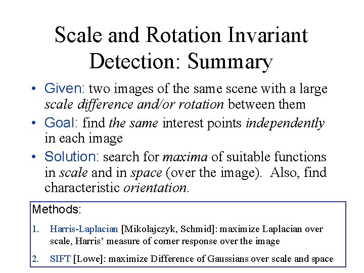
Scale and Rotation Invariant Detection: Summary • Given: two images of the same scene with a large scale difference and/or rotation between them • Goal: find the same interest points independently in each image • Solution: search for maxima of suitable functions in scale and in space (over the image). Also, find characteristic orientation. Methods: 1. Harris-Laplacian [Mikolajczyk, Schmid]: maximize Laplacian over scale, Harris’ measure of corner response over the image 2. SIFT [Lowe]: maximize Difference of Gaussians over scale and space

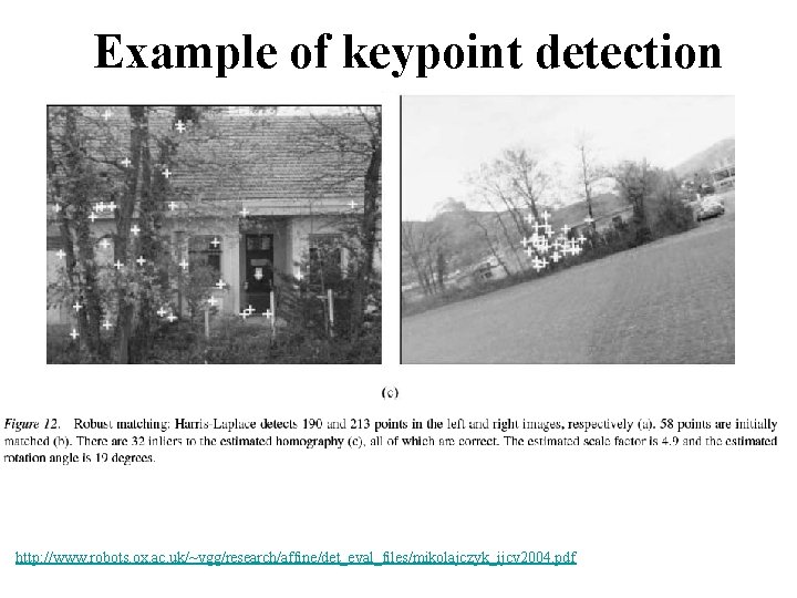
Example of keypoint detection http: //www. robots. ox. ac. uk/~vgg/research/affine/det_eval_files/mikolajczyk_ijcv 2004. pdf

Outline • Feature point detection – Harris corner detector – finding a characteristic scale • Local image description – SIFT features 123

Recall: Matching with Features • Problem 1: – Detect the same point independently in both images no chance to match! Good We need a repeatable detector

Recall: Matching with Features • Problem 2: – For each point correctly recognize the corresponding one ? We need a reliable and distinctive descriptor

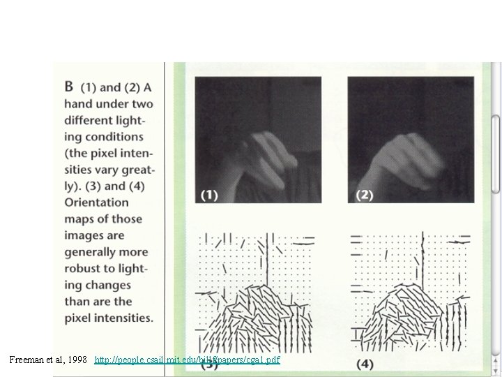
Freeman et al, 1998 http: //people. csail. mit. edu/billf/papers/cga 1. pdf

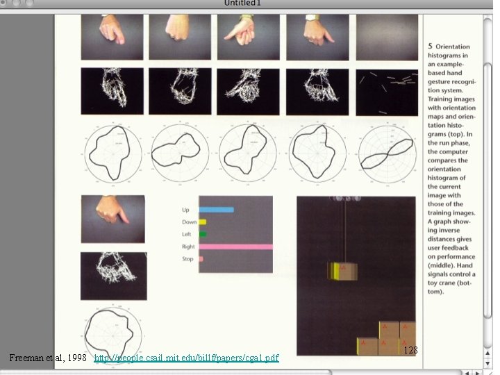
Freeman et al, 1998 http: //people. csail. mit. edu/billf/papers/cga 1. pdf 128

CVPR 2003 Tutorial Recognition and Matching Based on Local Invariant Features David Lowe Computer Science Department University of British Columbia http: //www. cs. ubc. ca/~lowe/papers/ijcv 04. pdf

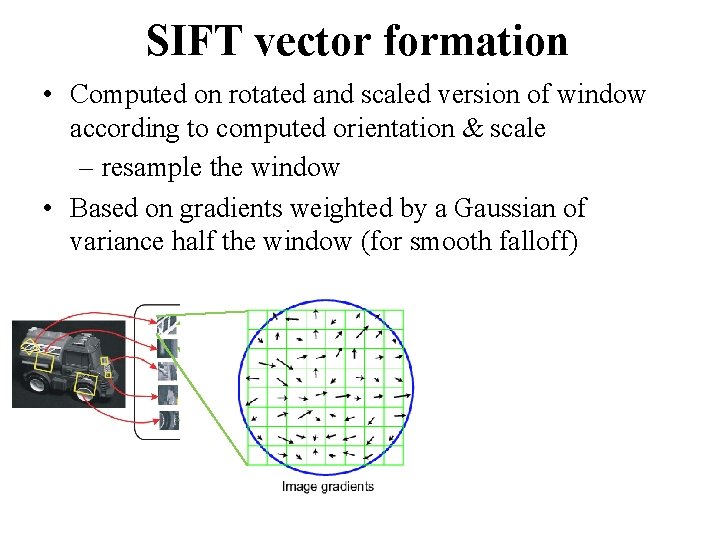
SIFT vector formation • Computed on rotated and scaled version of window according to computed orientation & scale – resample the window • Based on gradients weighted by a Gaussian of variance half the window (for smooth falloff)

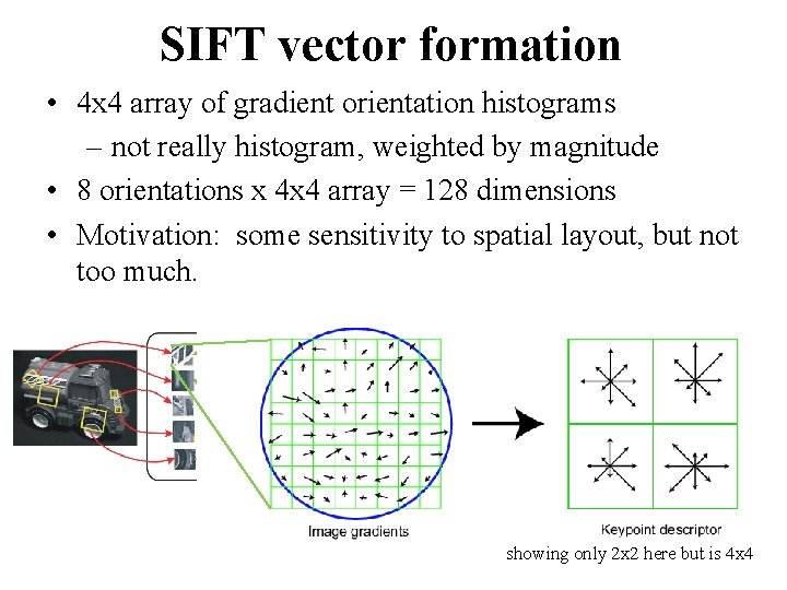
SIFT vector formation • 4 x 4 array of gradient orientation histograms – not really histogram, weighted by magnitude • 8 orientations x 4 x 4 array = 128 dimensions • Motivation: some sensitivity to spatial layout, but not too much. showing only 2 x 2 here but is 4 x 4

Reduce effect of illumination • 128 -dim vector normalized to 1 • Threshold gradient magnitudes to avoid excessive influence of high gradients – after normalization, clamp gradients >0. 2 – renormalize

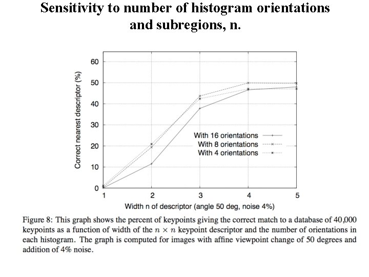
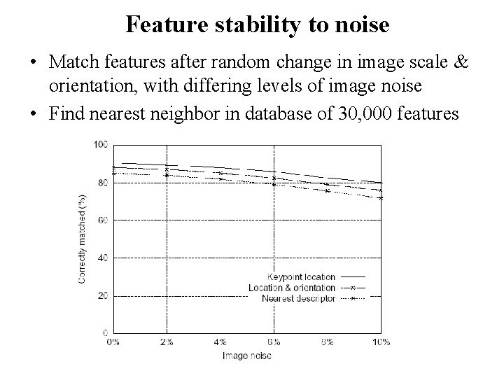
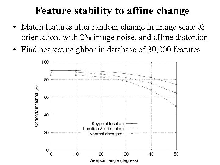
Tuning and evaluating the SIFT descriptors Database images were subjected to rotation, scaling, affine stretch, brightness and contrast changes, and added noise. Feature point detectors and descriptors were compared before and after the distortions, and evaluated for: • Sensitivity to number of histogram orientations and subregions. • Stability to noise. • Stability to affine change. • Feature distinctiveness 136

Sensitivity to number of histogram orientations and subregions, n.

Feature stability to noise • Match features after random change in image scale & orientation, with differing levels of image noise • Find nearest neighbor in database of 30, 000 features

Feature stability to affine change • Match features after random change in image scale & orientation, with 2% image noise, and affine distortion • Find nearest neighbor in database of 30, 000 features

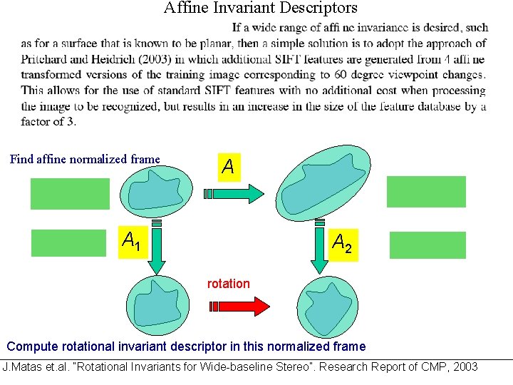
Affine Invariant Descriptors Find affine normalized frame A A 1 A 2 rotation Compute rotational invariant descriptor in this normalized frame J. Matas et. al. “Rotational Invariants for Wide-baseline Stereo”. Research Report of CMP, 2003

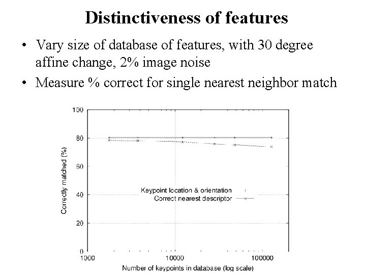
Distinctiveness of features • Vary size of database of features, with 30 degree affine change, 2% image noise • Measure % correct for single nearest neighbor match

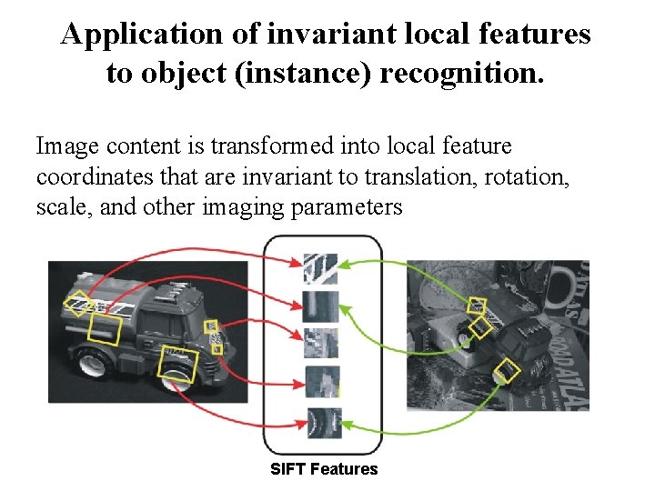
Application of invariant local features to object (instance) recognition. Image content is transformed into local feature coordinates that are invariant to translation, rotation, scale, and other imaging parameters SIFT Features


SIFT features impact SIFT feature paper citations: Distinctive image features from scale-invariant keypoints. DG Lowe International journal of computer vision, 2004 - Springer International Journal of Computer Vision 60(2), 91– 110, 2004 cс 2004 Kluwer Academic Publishers. Computer Science Department, University of British Columbia. . . Cited by 6537 A good SIFT features tutorial: http: //www. cs. toronto. edu/~jepson/csc 2503/tut. SIFT 04. pdf By Estrada, Jepson, and Fleet. The original SIFT paper: http: //www. cs. ubc. ca/~lowe/papers/ijcv 04. pdf

Now we have • Well-localized feature points • Distinctive descriptor • Now we need to – match pairs of feature points in different images – Robustly compute homographies (in the presence of errors/outliers)