Systematic force field optimization for more accurate molecular

Systematic force field optimization for more accurate molecular simulations Lee-Ping Wang Stanford Department of Chemistry Open. MM Workshop, Stanford University September 7, 2012

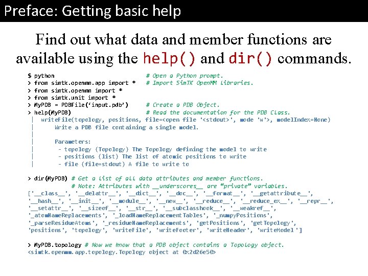
Preface: Getting basic help Find out what data and member functions are available using the help() and dir() commands. $ > > > python # Open a Python prompt. from simtk. openmm. app import * # Import Sim. TK Open. MM libraries. from simtk. openmm import * from simtk. unit import * My. PDB = PDBFile(‘input. pdb’) # Create a PDB Object. help(My. PDB) # Read the documentation for the PDB Class. | write. File(topology, positions, file=<open file '<stdout>', mode 'w'>, model. Index=None) | Write a PDB file containing a single model. | | Parameters: | - topology (Topology) The Topology defining the model to write | - positions (list) The list of atomic positions to write | - file (file=stdout) A file to write to > dir(My. PDB) # Get a list of all data attributes and member functions. # Note: Attributes with __underscores__ are “private” variables. ['__class__', '__delattr__', '__dict__', '__doc__', '__format__', '__getattribute__', '__hash__', '__init__', '__module__', '__new__', '__reduce_ex__', '__repr__', '__setattr__', '__sizeof__', '__str__', '__subclasshook__', '__weakref__', '_atom. Name. Replacements', '_load. Name. Replacement. Tables', '_numpy. Positions', '_parse. Residue. Atoms', '_residue. Name. Replacements', 'get. Positions', 'get. Topology', 'positions', 'topology', 'write. File', 'write. Footer', 'write. Header', 'write. Model '] > My. PDB. topology # Now we know that a PDB object contains a Topology object. <simtk. openmm. app. topology. Topology object at 0 x 2 d 26 e 50>

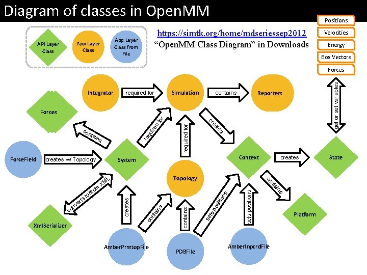
Diagram of classes in Open. MM https: //simtk. org/home/mdseriessep 2012 “Open. MM Class Diagram” in Downloads App Layer Class from File App Layer Class API Layer Class Positions Velocities Energy Box Vectors Integrator Simulation required for get or set variables Forces Reporters contains required for d ire re qu sets positions s ion ts po sit PDBFile se contains ain s nt co creates Amber. Prmtop. File Amber. Inpcrd. File ns Xml. Serializer ai co nt rts Topology L XM creates co m fro e nv Context System creates w/ Topology / to s Force. Field ins te nta ea co cr fo r Forces Platform State

Outline Introduction • Force fields in molecular mechanics • The ingredients of a force field • Functional form • Reference data • Optimization method Force. Balance program force field optimization • Overview of program • Application: Polarizable water model • Results and discussion • Basic program usage

Introduction: A wide range of simulation domains Single-point, 2 -3 atoms • Computer simulations of atoms and molecules span a vast range of detail 100 fs, 10 atoms: photochemistry 10 ms, thousands of atoms: protein folding, drug binding 1 ms+, 1 million atoms: dynamics of large proteins, cell membranes, viruses 10 ps, 100 atoms: chemical reactions • More detailed theories can describe complex phenomena and offer higher accuracy • Less detailed theories allow for simulation of larger systems / longer timescales • In molecular mechanics simulation, the potential energy of molecules is represented using an empirical force field

Introduction: Force Fields • Force fields are built from functional forms and empirical parameters • Interactions include bonded pairwise, 3 body, and 4 -body interactions… • … as well as nonbonded pairwise interactions • Simulation accuracy depends critically on choice of parameters

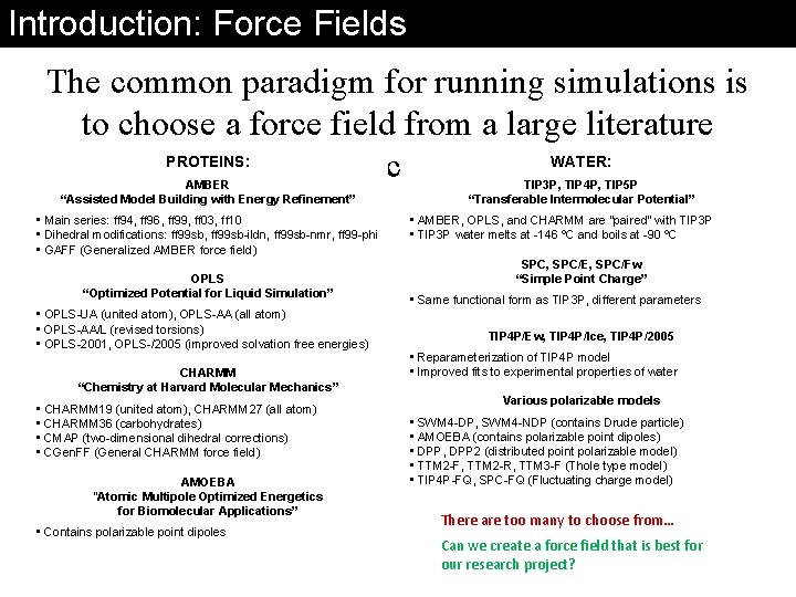
Introduction: Force Fields The common paradigm for running simulations is to choose a force field from a large literature PROTEINS: WATER: selection. AMBER “Assisted Model Building with Energy Refinement” • Main series: ff 94, ff 96, ff 99, ff 03, ff 10 • Dihedral modifications: ff 99 sb, ff 99 sb-ildn, ff 99 sb-nmr, ff 99 -phi • GAFF (Generalized AMBER force field) OPLS “Optimized Potential for Liquid Simulation” • OPLS-UA (united atom), OPLS-AA (all atom) • OPLS-AA/L (revised torsions) • OPLS-2001, OPLS-/2005 (improved solvation free energies) CHARMM “Chemistry at Harvard Molecular Mechanics” • CHARMM 19 (united atom), CHARMM 27 (all atom) • CHARMM 36 (carbohydrates) • CMAP (two-dimensional dihedral corrections) • CGen. FF (General CHARMM force field) AMOEBA “Atomic Multipole Optimized Energetics for Biomolecular Applications” • Contains polarizable point dipoles TIP 3 P, TIP 4 P, TIP 5 P “Transferable Intermolecular Potential” • AMBER, OPLS, and CHARMM are “paired” with TIP 3 P • TIP 3 P water melts at -146 ºC and boils at -90 ºC SPC, SPC/E, SPC/Fw “Simple Point Charge” • Same functional form as TIP 3 P, different parameters TIP 4 P/Ew, TIP 4 P/Ice, TIP 4 P/2005 • Reparameterization of TIP 4 P model • Improved fits to experimental properties of water Various polarizable models • SWM 4 -DP, SWM 4 -NDP (contains Drude particle) • AMOEBA (contains polarizable point dipoles) • DPP, DPP 2 (distributed point polarizable model) • TTM 2 -F, TTM 2 -R, TTM 3 -F (Thole type model) • TIP 4 P-FQ, SPC-FQ (Fluctuating charge model) There are too many to choose from… Can we create a force field that is best for our research project?

Creating a force field: Functional form Step 1: Choose a functional form to represent the potential energy surface, or design your own. AMBER fixed-charge force field: • Point charge on each atom AMOEBA polarizable force field: • Point charge, dipole, and quadrupole on each atom • Polarizable point dipole on each atom with short-range damping

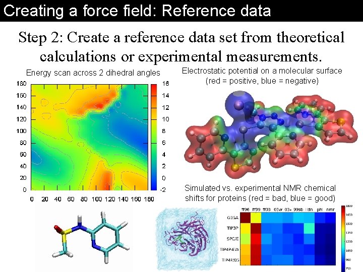
Creating a force field: Reference data Step 2: Create a reference data set from theoretical calculations or experimental measurements. Energy scan across 2 dihedral angles Electrostatic potential on a molecular surface (red = positive, blue = negative) Simulated vs. experimental NMR chemical shifts for proteins (red = bad, blue = good)

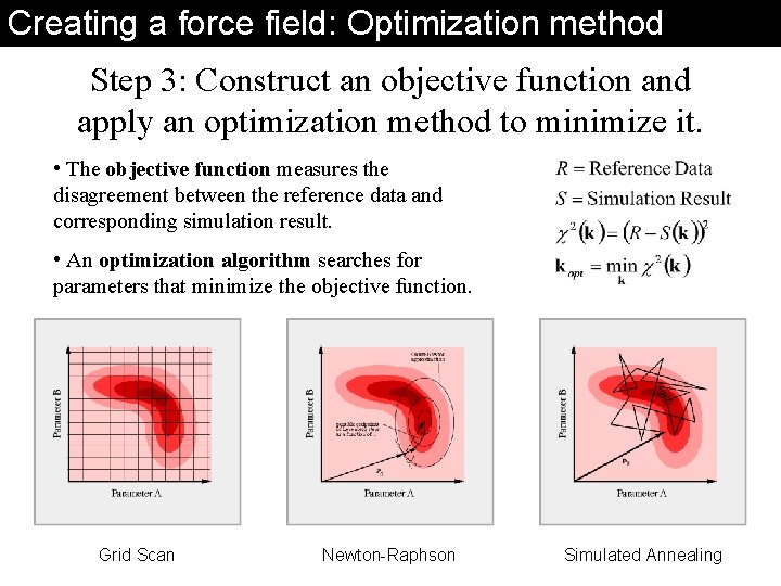
Creating a force field: Optimization method Step 3: Construct an objective function and apply an optimization method to minimize it. • The objective function measures the disagreement between the reference data and corresponding simulation result. • An optimization algorithm searches for parameters that minimize the objective function. Grid Scan Newton-Raphson Simulated Annealing

Outline Introduction • Force fields in molecular mechanics • The ingredients of a force field • Functional form • Reference data • Optimization method Force. Balance program force field optimization • Overview of program • Application: Polarizable water model • Results and discussion • Basic program usage

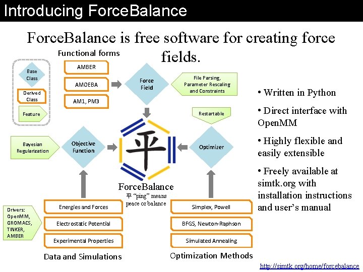
Introducing Force. Balance is free software for creating force Functional forms fields. AMBER Base Class Derived Class File Parsing, Parameter Rescaling and Constraints Force Field AMOEBA AM 1, PM 3 Restartable Feature Bayesian Regularization Objective Function Optimizer Force. Balance Drivers: Open. MM, GROMACS, TINKER, AMBER Energies and Forces 平 “ping” means peace or balance Simplex, Powell Electrostatic Potential BFGS, Newton-Raphson Experimental Properties Simulated Annealing Data and Simulations Optimization Methods • Written in Python • Direct interface with Open. MM • Highly flexible and easily extensible • Freely available at simtk. org with installation instructions and user’s manual http: //simtk. org/home/forcebalance

Polarizable water - motivation We applied Force. Balance to parameterize a variation on the AMOEBA water model. • The AMOEBA force field contains mutually induced dipoles • Direct induced dipoles are cheaper (5 x faster) but the physics of the model are different • 19 total tunable parameters

Polarizable water - results Our optimized model exceeds the accuracy of AMOEBA for several properties of water. • We used a large set of experimental and theoretical data: Property AMOEBA This work Experiment m-3) 1000 ± 1 999 ± 1 997 mol-1) 43. 8 ± 0. 1 44. 0 81 ± 10 81 ± 5 78. 4 2. 0 ± 0. 1 2. 3 15 - 25 0 - 10 4 Density (kg DHvap (k. J Dielectric constant Diffusion constant (10 -5 Density maximum (ºC) cm 2 s-1) 1) Energies and forces for 12, 000 geometries from QM theory 2) Gas-phase cluster binding energies from QM theory 3) Experimental monomer geometry, vibrational modes, and multipole moments 4) Experimental density and heat of vaporization curves • Fitted properties exceed accuracy of original AMOEBA • Other properties were also predicted

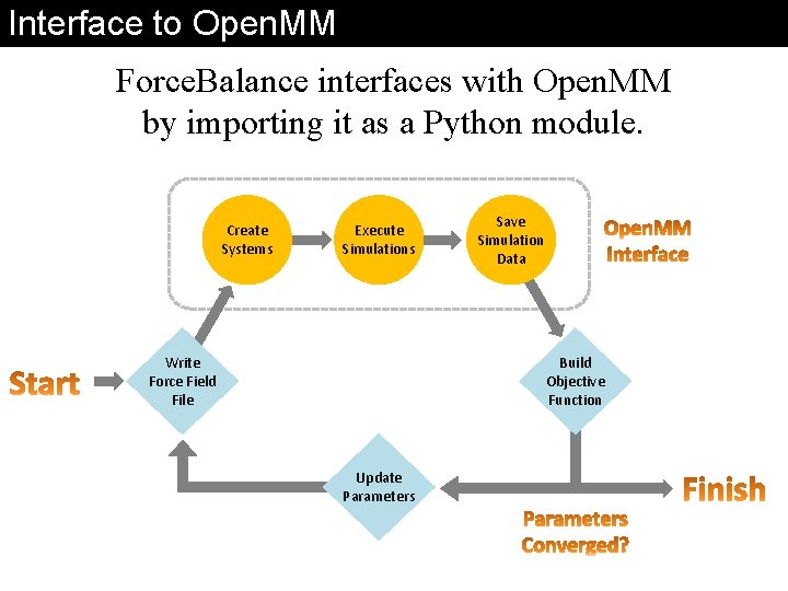
Interface to Open. MM Force. Balance interfaces with Open. MM by importing it as a Python module. Create Systems Execute Simulations Write Force Field File Save Simulation Data Build Objective Function Update Parameters

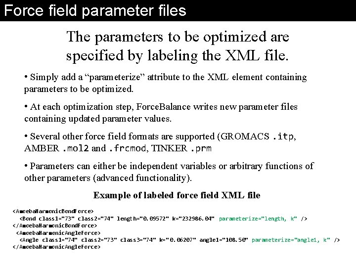
Force field parameter files The parameters to be optimized are specified by labeling the XML file. • Simply add a “parameterize” attribute to the XML element containing parameters to be optimized. • At each optimization step, Force. Balance writes new parameter files containing updated parameter values. • Several other force field formats are supported (GROMACS. itp, AMBER. mol 2 and. frcmod, TINKER. prm • Parameters can either be independent variables or arbitrary functions of other parameters (advanced functionality). Example of labeled force field XML file <Amoeba. Harmonic. Bond. Force> <Bond class 1="73" class 2="74" length="0. 09572" k="232986. 04" parameterize="length, k" /> </Amoeba. Harmonic. Bond. Force> <Amoeba. Harmonic. Angle. Force> <Angle class 1="74" class 2="73" class 3="74" k=" 0. 06207" angle 1="108. 50" parameterize="angle 1, k" /> </Amoeba. Harmonic. Angle. Force>

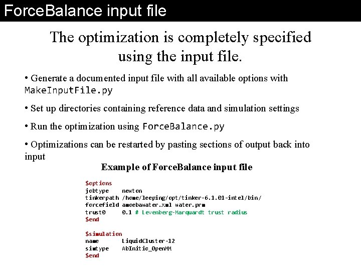
Force. Balance input file The optimization is completely specified using the input file. • Generate a documented input file with all available options with Make. Input. File. py • Set up directories containing reference data and simulation settings • Run the optimization using Force. Balance. py • Optimizations can be restarted by pasting sections of output back into input Example of Force. Balance input file $options jobtype tinkerpath forcefield trust 0 $end newton /home/leeping/opt/tinker-6. 1. 01 -intel/bin / amoebawater. xml water. prm 0. 1 # Levenberg-Marquardt trust radius $simulation name Liquid. Cluster-12 simtype Ab. Initio_Open. MM $end

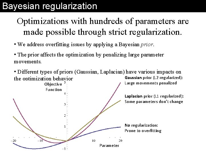
Bayesian regularization Optimizations with hundreds of parameters are made possible through strict regularization. • We address overfitting issues by applying a Bayesian prior. • The prior affects the optimization by penalizing large parameter movements. • Different types of priors (Gaussian, Laplacian) have various impacts on Gaussian prior (L 2 regularized): the optimization behavior Large movements penalized Objective Function Laplacian prior (L 1 regularized): Some parameters don’t change No regularization: Prone to overfitting Parameter

Conclusion We hope that Force. Balance will systematize and democratize the discipline of force field development. Systematic optimization methods: • Optimize parameters using theoretical and experimental data simultaneously • Parameterization calculations are reproducible and systematically improvable • Rigorously prevent overfitting using strict regularization methods Give everybody the infrastructure for making good force fields: • Improve simulation accuracy for uncommon (non-mainstream) molecules, where force field development efforts are relatively sparse • All-inclusive: New interfaces with simulation software easy to write • Reduce the headache of force field development and let’shttp: //simtk. org/home/forcebalance focus on the