Systematic Bounding Techniques for Combinatorial Optimization Sharlee Climer

Systematic Bounding Techniques for Combinatorial Optimization Sharlee Climer and Weixiong Zhang Department of Computer Science and Engineering Washington University in St. Louis This research was funded in part by NDSEG and Olin Fellowships, NSF grants IIS-0196057 and ITR/EIA-0113618, and in part by DARPA Cooperative Agreement F 30602 -00 -2 -0531. AAAI-05 Tutorial Bounding Techniques

Overview n Introduction n Formulation and notation n Historical perspective n Modifications to obtain bounds n Two-step procedure n Exploiting the use of bounds n Future directions AAAI-05 Tutorial Bounding Techniques 2

What is the “use of bounds”? AAAI-05 Tutorial Bounding Techniques 3

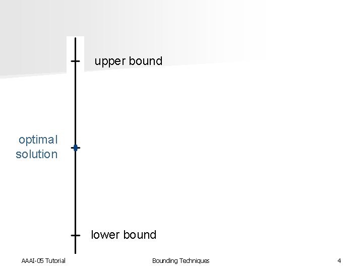
upper bound optimal solution lower bound AAAI-05 Tutorial Bounding Techniques 4

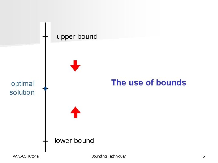
upper bound The use of bounds optimal solution lower bound AAAI-05 Tutorial Bounding Techniques 5

Use of bounds n n n Bounds have been extensively studied in both computer science and operations research (OR) Pruning rules in branch-and-bound search Without the use of bounds, many important problems would be unsolvable Previous efforts to systematically discover effective relaxations to be used for bounds Recent work to systematically discover other modifications for use as bounds AAAI-05 Tutorial Bounding Techniques 6

Objectives of tutorial n Survey the previous uses of bounds n Reorganize existing work in a systematic way n Point out potential directions for future work AAAI-05 Tutorial Bounding Techniques 7

Formulation and notation n Techniques presented can be applied to a variety of optimization problems n To demonstrate the use of bounds, we’ll use integer linear programs (IPs) as basic problem structure n Without loss of generality, we consider only minimization problems AAAI-05 Tutorial Bounding Techniques 8

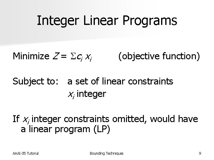
Integer Linear Programs Minimize Z = Sci xi (objective function) Subject to: a set of linear constraints xi integer If xi integer constraints omitted, would have a linear program (LP) AAAI-05 Tutorial Bounding Techniques 9

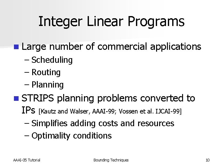
Integer Linear Programs n Large number of commercial applications – Scheduling – Routing – Planning n STRIPS planning problems converted to IPs [Kautz and Walser, AAAI-99; Vossen et al. IJCAI-99] – Simplifies adding costs and resources – Optimality conditions AAAI-05 Tutorial Bounding Techniques 10

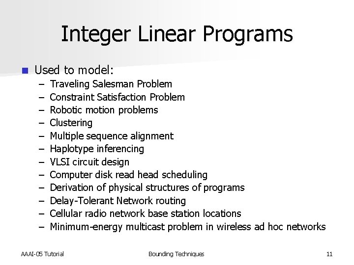
Integer Linear Programs n Used to model: – – – Traveling Salesman Problem Constraint Satisfaction Problem Robotic motion problems Clustering Multiple sequence alignment Haplotype inferencing VLSI circuit design Computer disk read head scheduling Derivation of physical structures of programs Delay-Tolerant Network routing Cellular radio network base station locations Minimum-energy multicast problem in wireless ad hoc networks AAAI-05 Tutorial Bounding Techniques 11

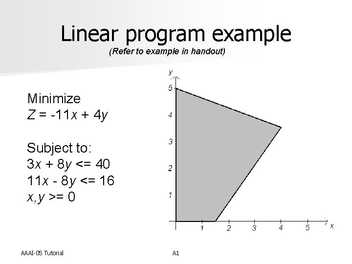
Linear program example (Refer to example in handout) Minimize Z = -11 x + 4 y Subject to: 3 x + 8 y <= 40 11 x - 8 y <= 16 x, y >= 0 AAAI-05 Tutorial A 1

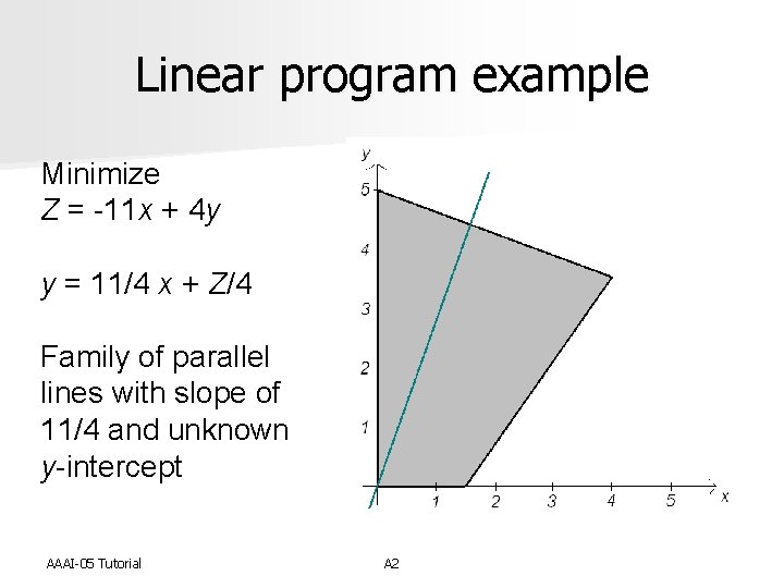
Linear program example Minimize Z = -11 x + 4 y y = 11/4 x + Z/4 Family of parallel lines with slope of 11/4 and unknown y-intercept AAAI-05 Tutorial A 2

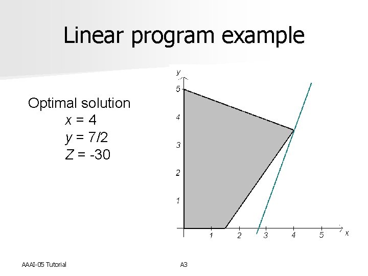
Linear program example Optimal solution x = 4 y = 7/2 Z = -30 AAAI-05 Tutorial A 3

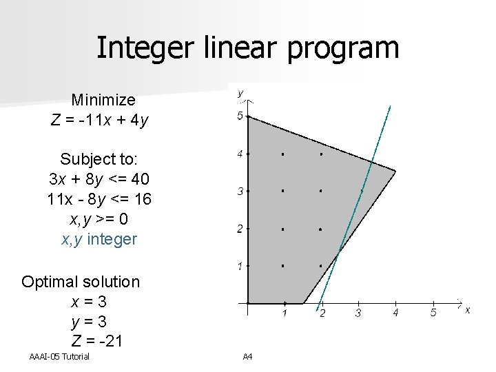
Integer linear program Minimize Z = -11 x + 4 y Subject to: 3 x + 8 y <= 40 11 x - 8 y <= 16 x, y >= 0 x, y integer Optimal solution x = 3 y = 3 Z = -21 AAAI-05 Tutorial A 4

Dual problem n Every IP has a dual problem that is also an IP n Original IP referred to as primal n If primal is a minimization IP, then dual is a maximization IP n Same coefficients, but rearranged n Inequalities in constraints are reversed AAAI-05 Tutorial A 5

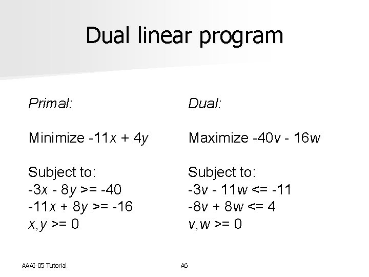
Dual linear program Primal: Dual: Minimize -11 x + 4 y Maximize -40 v - 16 w Subject to: -3 x - 8 y >= -40 -11 x + 8 y >= -16 x, y >= 0 Subject to: -3 v - 11 w <= -11 -8 v + 8 w <= 4 v, w >= 0 AAAI-05 Tutorial A 6

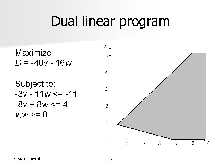
Dual linear program Maximize D = -40 v - 16 w Subject to: -3 v - 11 w <= -11 -8 v + 8 w <= 4 v, w >= 0 AAAI-05 Tutorial A 7

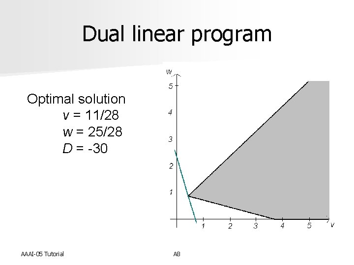
Dual linear program Optimal solution v = 11/28 w = 25/28 D = -30 AAAI-05 Tutorial A 8

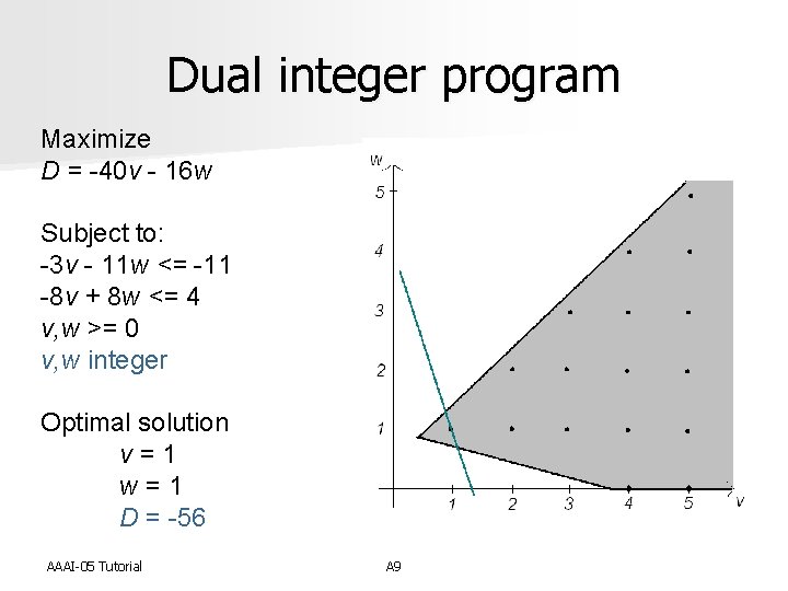
Dual integer program Maximize D = -40 v - 16 w Subject to: -3 v - 11 w <= -11 -8 v + 8 w <= 4 v, w >= 0 v, w integer Optimal solution v = 1 w = 1 D = -56 AAAI-05 Tutorial A 9

The Traveling Salesman Problem n The Traveling Salesman Problem (TSP) is the problem of finding a minimum cost complete tour of a set of cities n STSP: cost from city i to city j is equal to the cost from city j to city i n ATSP: costs not necessarily equal AAAI-05 Tutorial Bounding Techniques 21

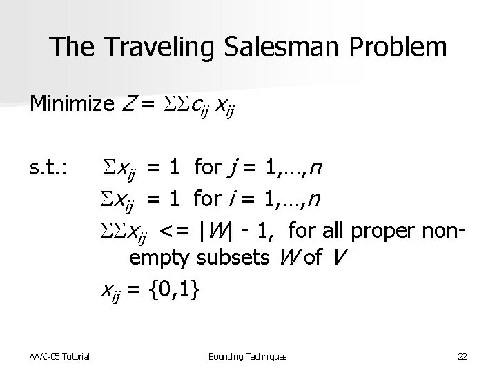
The Traveling Salesman Problem Minimize Z = SScij xij s. t. : Sxij = 1 for j = 1, …, n Sxij = 1 for i = 1, …, n SSxij <= |W| - 1, for all proper non- empty subsets W of V xij = {0, 1} AAAI-05 Tutorial Bounding Techniques 22

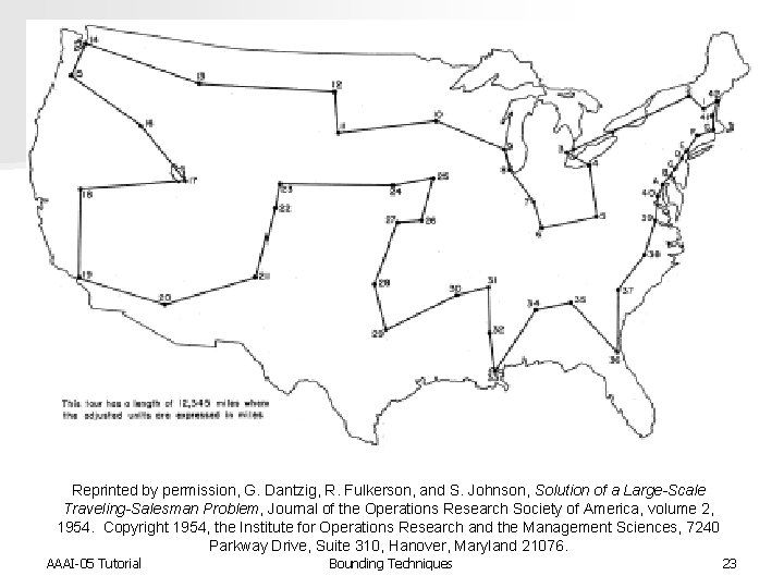
Reprinted by permission, G. Dantzig, R. Fulkerson, and S. Johnson, Solution of a Large-Scale Traveling-Salesman Problem, Journal of the Operations Research Society of America, volume 2, 1954. Copyright 1954, the Institute for Operations Research and the Management Sciences, 7240 Parkway Drive, Suite 310, Hanover, Maryland 21076. AAAI-05 Tutorial Bounding Techniques 23

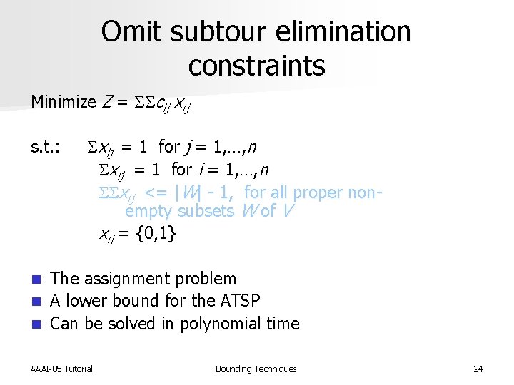
Omit subtour elimination constraints Minimize Z = SScij xij s. t. : Sxij = 1 for j = 1, …, n Sxij = 1 for i = 1, …, n SSxij <= |W| - 1, for all proper non- empty subsets W of V xij = {0, 1} The assignment problem n A lower bound for the ATSP n Can be solved in polynomial time n AAAI-05 Tutorial Bounding Techniques 24

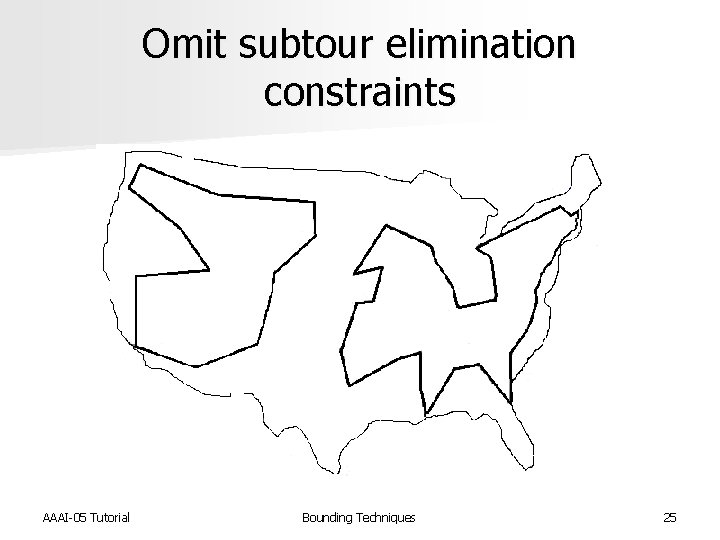
Omit subtour elimination constraints AAAI-05 Tutorial Bounding Techniques 25

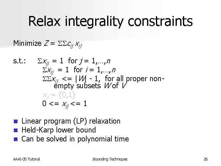
Relax integrality constraints Minimize Z = SScij xij s. t. : Sxij = 1 for j = 1, …, n Sxij = 1 for i = 1, …, n SSxij <= |W| - 1, for all proper non- empty subsets W of V xij = {0, 1} 0 <= xij <= 1 n n n Linear program (LP) relaxation Held-Karp lower bound Can be solved in polynomial time AAAI-05 Tutorial Bounding Techniques 26

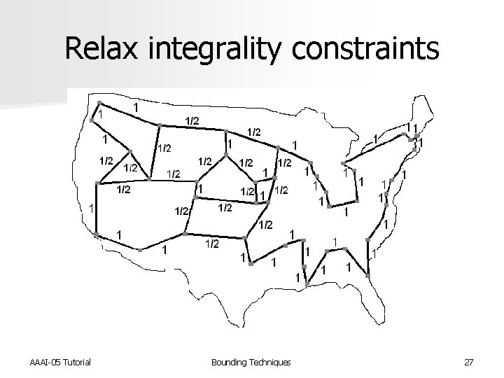
Relax integrality constraints AAAI-05 Tutorial Bounding Techniques 27

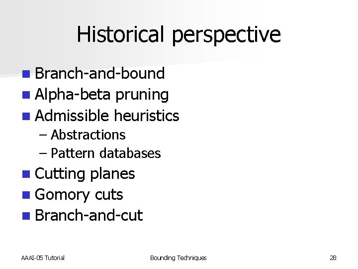
Historical perspective n Branch-and-bound n Alpha-beta pruning n Admissible heuristics – Abstractions – Pattern databases n Cutting planes n Gomory cuts n Branch-and-cut AAAI-05 Tutorial Bounding Techniques 28

Branch-and-bound n In 1958, several papers appeared using branchand-bound (Bn. B) [Bock, Op. Res. 1958; Croes, Op. Res. 1958; Eastman, Ph. D thesis 1958, Rossman and Twery, Op. Res. 1958] Three of these papers introduced algorithms for the TSP n “Branch-and-bound” coined [Little et al. Op. Res. 1963] (also a TSP algorithm) n Example: Carpaneto, Dell’Amico, and Toth’s (CDT) algorithm for the ATSP [ACM Trans. On Math. n Software 1995] AAAI-05 Tutorial Bounding Techniques 29

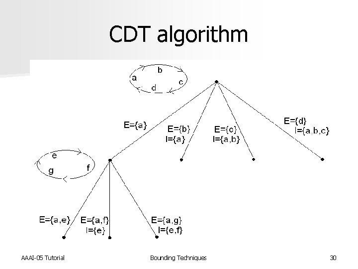
CDT algorithm AAAI-05 Tutorial Bounding Techniques 30

Branch-and-bound n Croes TSP algorithm perhaps first Bn. B search published [Croes, Op. Res. 1958] n Used bounds in two different ways n Found an approximate solution n Used solution as upper bound for eliminating sets of arcs that cannot simultaneously appear n Bn. B tree over remaining arc combinations AAAI-05 Tutorial Bounding Techniques 31

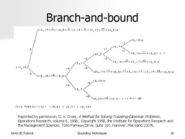
Branch-and-bound Reprinted by permission, G. A. Croes, A Method for Solving Traveling-Salesman Problems, Operations Research, volume 6, 1958. Copyright 1958, the Institute for Operations Research and the Management Sciences, 7240 Parkway Drive, Suite 310, Hanover, Maryland 21076. AAAI-05 Tutorial Bounding Techniques 32

Branch-and-bound n Croes solved 49 -city STSP that had previously been solved by Dantzig, Fulkerson, and Johnson [Op. Res. 1954] n Improvements: – Mechanized solver – Provides “anytime” solution – Faster than previous methods n Croes solved by hand – 70 hours to solve – Found optimal solution after 10 hours AAAI-05 Tutorial Bounding Techniques 33

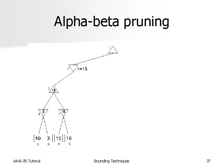
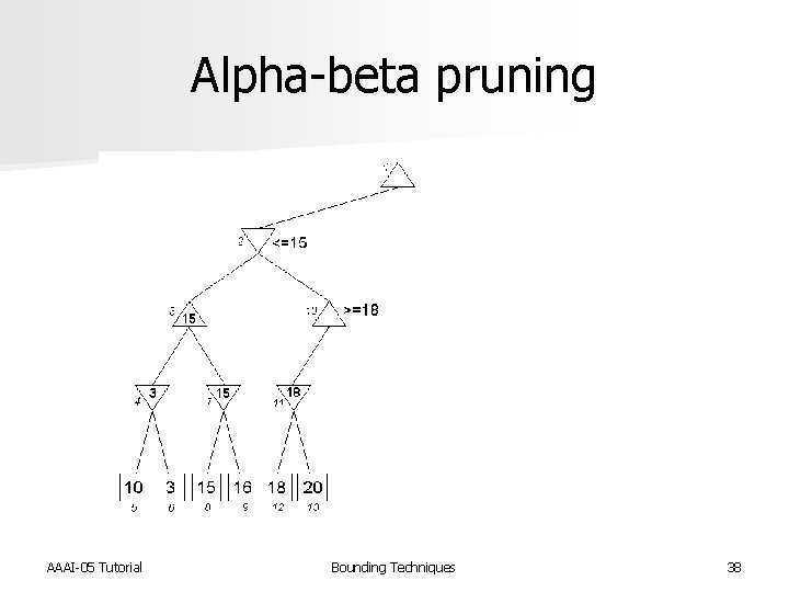
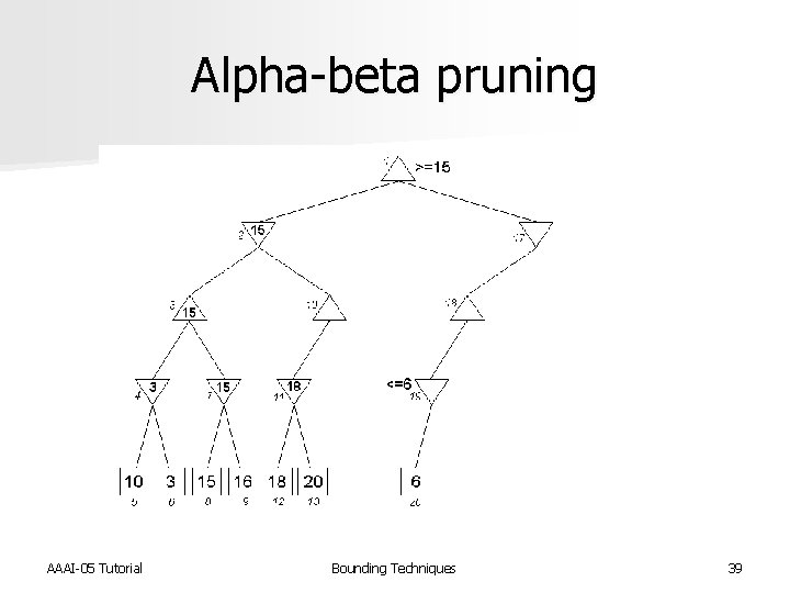
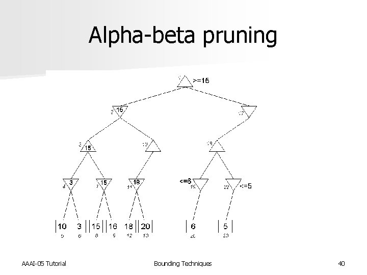
Alpha-beta pruning n Minimax search is a specialized Bn. B search for game playing n Objective is to determine the best move n Alpha-beta pruning used to reduce the number of nodes that need to be evaluated AAAI-05 Tutorial Bounding Techniques 34

Alpha-beta pruning n Devised by John Mc. Carthy in 1956, but not published n Used in the NSS chess program in 1958 [Newell et al. IBM Journal of R&D 1958] n Pearl proved alpha-beta to be an asymptotically optimal game-searching algorithm [Pearl, Comm. of ACM 1982] n Modified strategy used by Deep Blue [Hsu, Behind Deep Blue 2002] AAAI-05 Tutorial Bounding Techniques 35

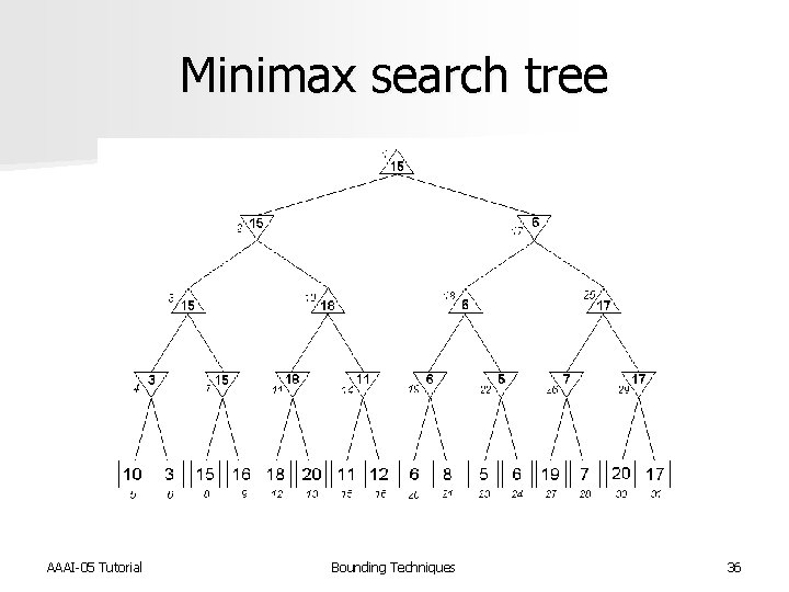
Minimax search tree AAAI-05 Tutorial Bounding Techniques 36

Alpha-beta pruning AAAI-05 Tutorial Bounding Techniques 37

Alpha-beta pruning AAAI-05 Tutorial Bounding Techniques 38

Alpha-beta pruning AAAI-05 Tutorial Bounding Techniques 39

Alpha-beta pruning AAAI-05 Tutorial Bounding Techniques 40

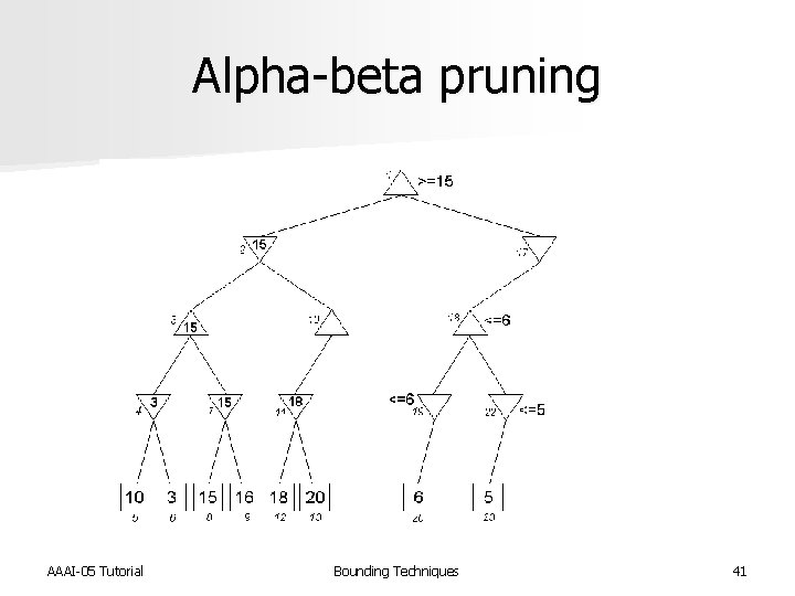
Alpha-beta pruning AAAI-05 Tutorial Bounding Techniques 41

Alpha-beta pruning AAAI-05 Tutorial Bounding Techniques 42

Admissible heuristics n Evaluation functions used by minimax are examples of heuristics n Trade-off of accuracy vs. time to compute n Admissible heuristic provides a lower bound n Admissibility needed to guarantee A* search performance n Admissibility allows pruning AAAI-05 Tutorial Bounding Techniques 43

Admissible heuristics Abstractions used for admissible heuristics can be generated by relaxing constraints n In 1970, Held and Karp used relaxation for the STSP [Op. Res. 1970] n – – 1 -tree A spanning tree with an added edge Node 1 has degree two and is part of single cycle Find MST without node 1 and add two smallest edges incident to node 1 AAAI-05 Tutorial Bounding Techniques 44

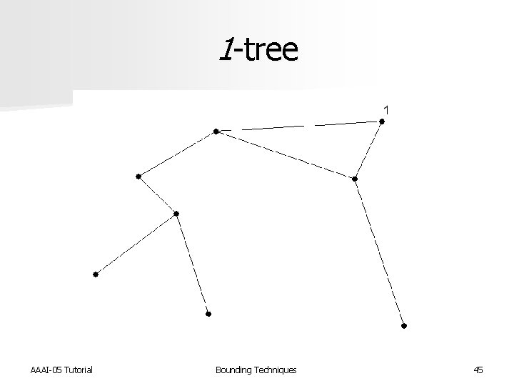
1 -tree AAAI-05 Tutorial Bounding Techniques 45

Systematic generation In 1982, Pearl suggested automatically deriving admissible heuristics by systematically deleting constraints* [Pearl, reprinted in AI Magazine 1983] n Absolver II [Prieditis, Machine Learning 1993] n – An implementation to automatically derive admissible heuristics – Uses abstracting transformations § Reduces cost function and/or § Expands goal states – Used to find first useful heuristic for Rubik’s cube * Introduced earlier by Somalvico et al. AAAI-05 Tutorial Bounding Techniques 46

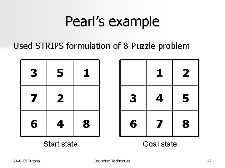
Pearl’s example Used STRIPS formulation of 8 -Puzzle problem 3 5 7 2 6 4 1 8 1 2 3 4 5 6 7 8 Start state AAAI-05 Tutorial Goal state Bounding Techniques 47

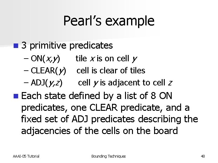
Pearl’s example n 3 primitive predicates – ON(x, y) tile x is on cell y – CLEAR(y) cell is clear of tiles – ADJ(y, z) cell y is adjacent to cell z n Each state defined by a list of 8 ON predicates, one CLEAR predicate, and a fixed set of ADJ predicates describing the adjacencies of the cells on the board AAAI-05 Tutorial Bounding Techniques 48

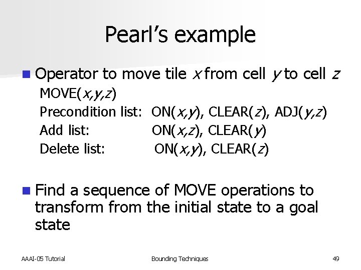
Pearl’s example n Operator to move tile x from cell y to cell z MOVE(x, y, z) Precondition list: ON(x, y), CLEAR(z), ADJ(y, z) Add list: ON(x, z), CLEAR(y) Delete list: ON(x, y), CLEAR(z) n Find a sequence of MOVE operations to transform from the initial state to a goal state AAAI-05 Tutorial Bounding Techniques 49

Pearl’s example n Removing CLEAR(z) and ADJ(y, z) from the precondition list – Permits a tile to be moved from its current position to any other position in one move – Equal to the number of tiles that are misplaced in initial state n Removing CLEAR(z) from the precondition list – Equals the sum of the Manhattan distances AAAI-05 Tutorial Bounding Techniques 50

Pearl’s example n n n Removing ADJ(y, z) from the precondition list Swap the blank with any other tile Can be solved with greedy algorithm – If current empty cell y is to be covered with tile x, move x to cell y. Else move any misplaced tile into y. Less intuitive than other two heuristics Discovered 13 years after A* was tested using the other two n Constraints can be divided n n – Tighter lower bound if only part of constraint is removed AAAI-05 Tutorial Bounding Techniques 51

Pattern databases n n n A look-up table containing precomputed solutions to subproblems Cost of solving entire problem is at least as large as cost of solving subproblem Large memory requirements Used to find first optimal solutions to random Rubik’s Cube [Korf, Workshop on Computer Games, IJCAI-97] Introduced by Culberson and Schaeffer and demonstrated on 15 -puzzle [Lecture Notes in AI, 1996] – Precomputed minimum cost for placing 7 tiles plus the “empty” tile in correct final position AAAI-05 Tutorial Bounding Techniques 52

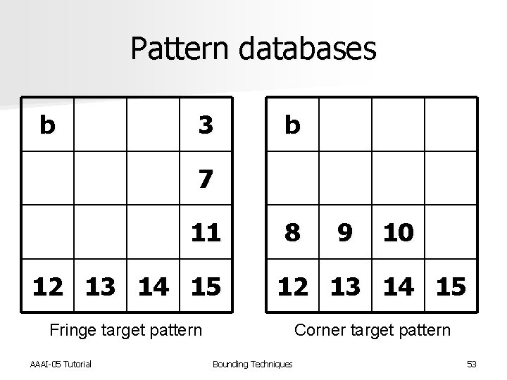
Pattern databases b 3 b 7 11 8 9 10 12 13 14 15 Fringe target pattern Corner target pattern AAAI-05 Tutorial Bounding Techniques 53

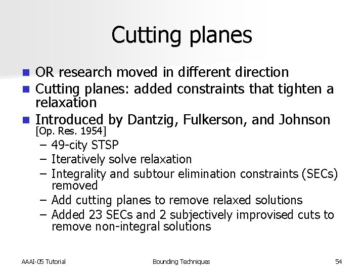
Cutting planes OR research moved in different direction Cutting planes: added constraints that tighten a relaxation n Introduced by Dantzig, Fulkerson, and Johnson n n [Op. Res. 1954] – – – 49 -city STSP Iteratively solve relaxation Integrality and subtour elimination constraints (SECs) removed – Add cutting planes to remove relaxed solutions – Added 23 SECs and 2 subjectively improvised cuts to remove non-integral solutions AAAI-05 Tutorial Bounding Techniques 54

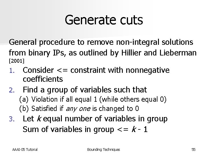
Generate cuts General procedure to remove non-integral solutions from binary IPs, as outlined by Hillier and Lieberman [2001] Consider <= constraint with nonnegative coefficients 2. Find a group of variables such that 1. (a) (b) 3. Violation if all equal 1 (while others equal 0) Satisfied if any one is changed to 0 Let k equal number of variables in group Sum of variables in group <= k - 1 AAAI-05 Tutorial Bounding Techniques 55

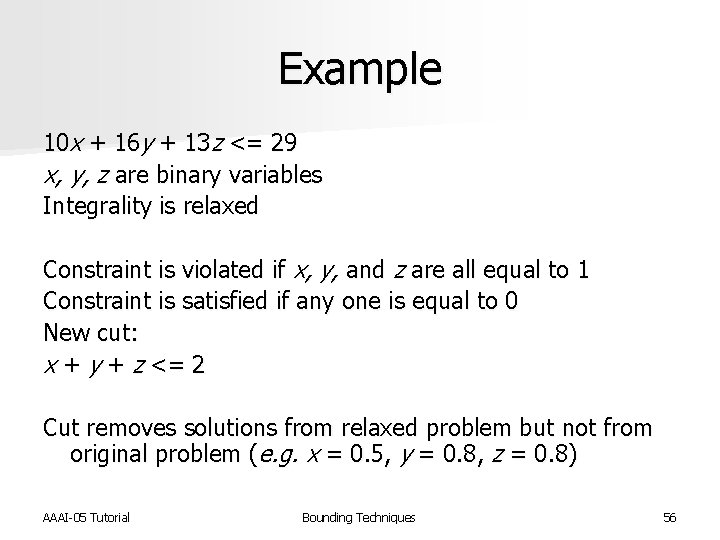
Example 10 x + 16 y + 13 z <= 29 x, y, z are binary variables Integrality is relaxed Constraint is violated if x, y, and z are all equal to 1 Constraint is satisfied if any one is equal to 0 New cut: x + y + z <= 2 Cut removes solutions from relaxed problem but not from original problem (e. g. x = 0. 5, y = 0. 8, z = 0. 8) AAAI-05 Tutorial Bounding Techniques 56

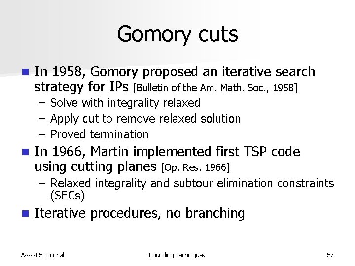
Gomory cuts n In 1958, Gomory proposed an iterative search strategy for IPs [Bulletin of the Am. Math. Soc. , 1958] – Solve with integrality relaxed – Apply cut to remove relaxed solution – Proved termination n In 1966, Martin implemented first TSP code using cutting planes [Op. Res. 1966] – Relaxed integrality and subtour elimination constraints (SECs) n Iterative procedures, no branching AAAI-05 Tutorial Bounding Techniques 57

Branch-and-cut n Branch-and-cut (Bn. C) is a Bn. B search with cutting planes added to relaxations at nodes n Hong implemented Bn. C code in 1972 for the TSP [Ph. D thesis, Johns Hopkins, 1972] n In 1987, Padberg and Rinaldi coined “branch-and-cut” and used to solve 532 city STSP [Op. Res. Letters 1987] AAAI-05 Tutorial Bounding Techniques 58

Concorde n In 1994, first implementation of Concorde n Branch-and-cut code for STSP Relaxed integrality and SECs Also used custom cuts tailored for the TSP Apply cuts at a node until diminishing returns Branch by setting value of an arc In 2004, Concorde was used to solve a 24, 978 city STSP [Applegate et al. www. tsp. gatech. edu] n n n [Applegate et al. Lecture Notes in Comp. Sci. 2001] – 14, 827, 429 cutting planes in addition to SECs AAAI-05 Tutorial Bounding Techniques 59

Modifications to obtain bounds n Many possibilities for obtaining bounds have been previously overlooked n Examine every aspect of problem description n Modifications of IPs to produce bounds – Relaxing or tightening constraints – Modifying objective function – Adding or deleting decision variables – Modifications to dual problem AAAI-05 Tutorial Bounding Techniques 60

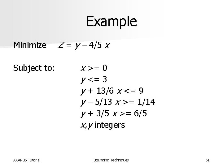
Example Minimize Z = y – 4/5 x Subject to: AAAI-05 Tutorial x >= 0 y <= 3 y + 13/6 x <= 9 y – 5/13 x >= 1/14 y + 3/5 x >= 6/5 x, y integers Bounding Techniques 61

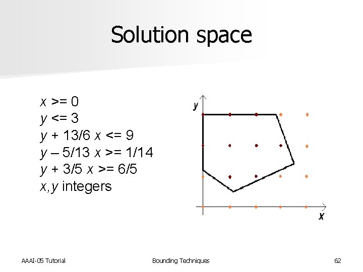
Solution space x >= 0 y <= 3 y + 13/6 x <= 9 y – 5/13 x >= 1/14 y + 3/5 x >= 6/5 x, y integers AAAI-05 Tutorial Bounding Techniques 62

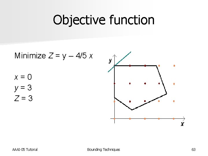
Objective function Minimize Z = y – 4/5 x x = 0 y = 3 Z = 3 AAAI-05 Tutorial Bounding Techniques 63

Optimal solution Minimize Z = y – 4/5 x x = 2 y = 1 Z = -0. 6 AAAI-05 Tutorial Bounding Techniques 64

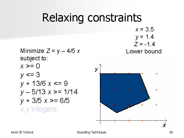
Relaxing constraints Minimize Z = y – 4/5 x subject to: x = 3. 5 y = 1. 4 Z = -1. 4 Lower bound x >= 0 y <= 3 y + 13/6 x <= 9 y – 5/13 x >= 1/14 y + 3/5 x >= 6/5 x, y integers AAAI-05 Tutorial Bounding Techniques 65

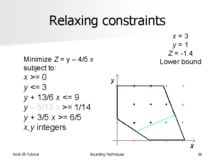
Relaxing constraints Minimize Z = y – 4/5 x subject to: x = 3 y = 1 Z = -1. 4 Lower bound x >= 0 y <= 3 y + 13/6 x <= 9 y – 5/13 x >= 1/14 y + 3/5 x >= 6/5 x, y integers AAAI-05 Tutorial Bounding Techniques 66

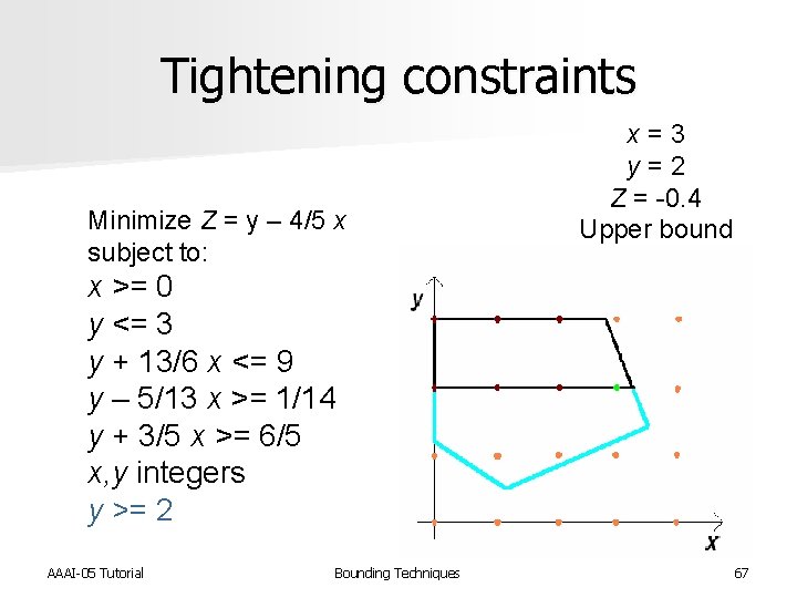
Tightening constraints Minimize Z = y – 4/5 x subject to: x = 3 y = 2 Z = -0. 4 Upper bound x >= 0 y <= 3 y + 13/6 x <= 9 y – 5/13 x >= 1/14 y + 3/5 x >= 6/5 x, y integers y >= 2 AAAI-05 Tutorial Bounding Techniques 67

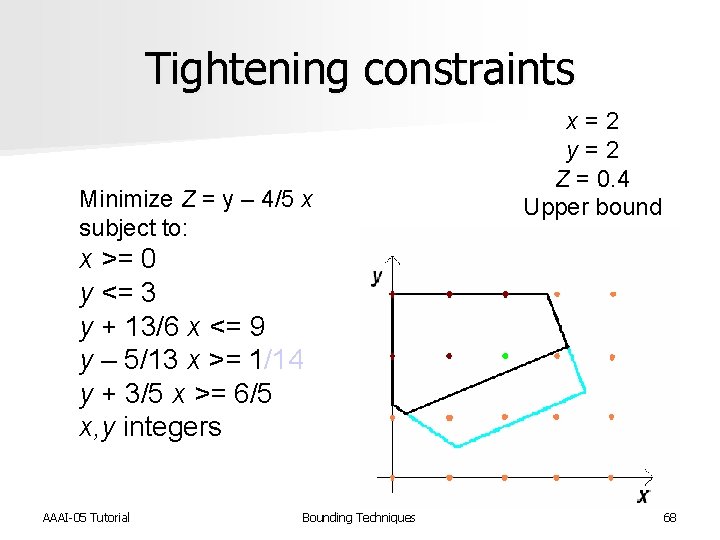
Tightening constraints Minimize Z = y – 4/5 x subject to: x = 2 y = 2 Z = 0. 4 Upper bound x >= 0 y <= 3 y + 13/6 x <= 9 y – 5/13 x >= 1/14 y + 3/5 x >= 6/5 x, y integers AAAI-05 Tutorial Bounding Techniques 68

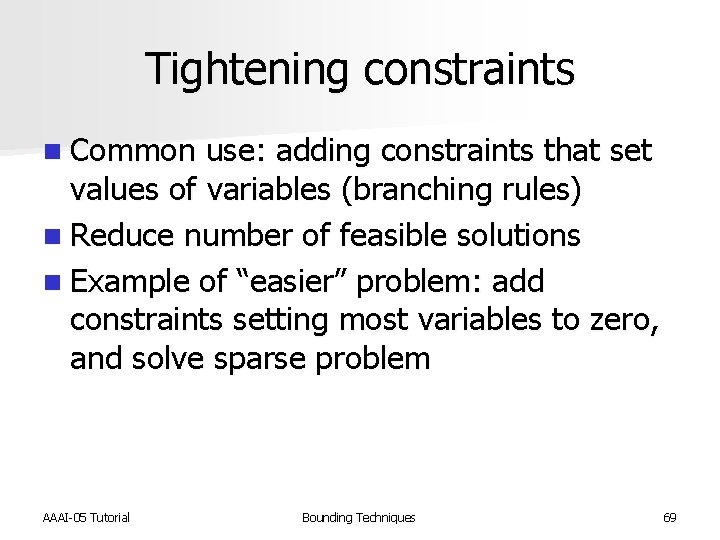
Tightening constraints n Common use: adding constraints that set values of variables (branching rules) n Reduce number of feasible solutions n Example of “easier” problem: add constraints setting most variables to zero, and solve sparse problem AAAI-05 Tutorial Bounding Techniques 69

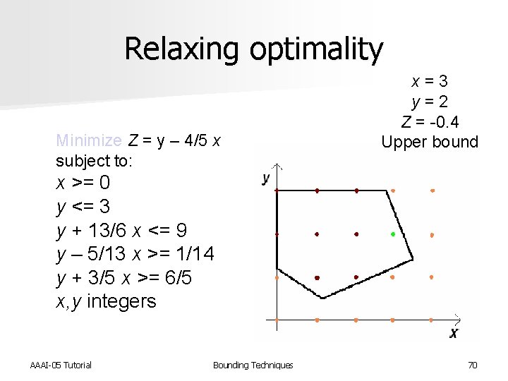
Relaxing optimality Minimize Z = y – 4/5 x subject to: x = 3 y = 2 Z = -0. 4 Upper bound x >= 0 y <= 3 y + 13/6 x <= 9 y – 5/13 x >= 1/14 y + 3/5 x >= 6/5 x, y integers AAAI-05 Tutorial Bounding Techniques 70

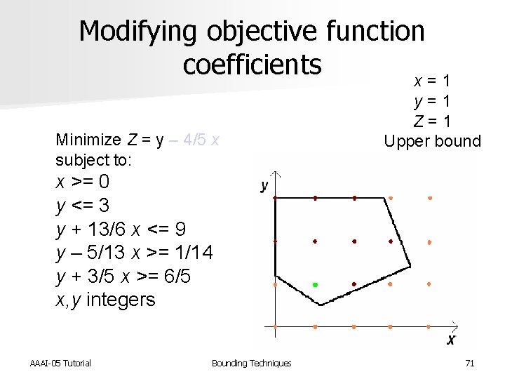
Modifying objective function coefficients x = 1 Minimize Z = y – 4/5 x subject to: y = 1 Z = 1 Upper bound x >= 0 y <= 3 y + 13/6 x <= 9 y – 5/13 x >= 1/14 y + 3/5 x >= 6/5 x, y integers AAAI-05 Tutorial Bounding Techniques 71

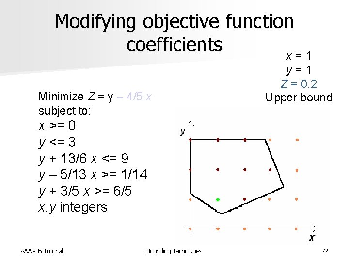
Modifying objective function coefficients x = 1 Minimize Z = y – 4/5 x subject to: y = 1 Z = 0. 2 Upper bound x >= 0 y <= 3 y + 13/6 x <= 9 y – 5/13 x >= 1/14 y + 3/5 x >= 6/5 x, y integers AAAI-05 Tutorial Bounding Techniques 72

Modifying objective function coefficients n Reducing range of objective function coefficients can yield “easier” problem for TSP n Phase transitions – difficulty in solving problem changes dramatically when a parameter is increased beyond a distinct value n For TSP, parameter is range of cij values AAAI-05 Tutorial Bounding Techniques 73

Modifying objective function coefficients n Zhang reduced range by eliminating least significant bits [CP-AI-OR-02] n After finding solution, used original values to compute cost of tour, yielding an upper bound n Could derive a lower bound by rounding values down and keeping these values when computing cost of tour found AAAI-05 Tutorial Bounding Techniques 74

Modifying objective function coefficients n Frieze’s polynomial-time STSP algorithm [SIAM Computing 1987] – Finds exact solution with a probability that tends to 1 as the number of cities n tends to infinity – Random cost values drawn from zero to B (n) - 1, where B (n) = o (n / log n) AAAI-05 Tutorial Bounding Techniques 75

Modifying objective function coefficients n Lagrangian relaxation – Adds penalties to objective function for violation of deleted constraints [Fisher, Management Science 1981] – Deletion of constraints yields lower bound – Addition of penalties tightens the bound, but it is still a lower bound – Can be used as a lower bound for pruning or as a heuristic to guide the search AAAI-05 Tutorial Bounding Techniques 76

Adding decision variables n Assuming zero is in allowable range for new variable n Addition of variable creates a lower bound n Creates additional feasible solutions, doesn’t exclude any feasible solutions to original problem n Example 1: add edges in graph problems – May create shortcuts AAAI-05 Tutorial Bounding Techniques 77

Adding decision variables n n Example 2: tilted drilling machine problems, a class of ATSPs Convert ATSP to STSP with 2 -node transformation Solved 800 100 -city instances using Concorde and ATSP solvers Number of decision variables more than quadrupled*, yet modified problems were generally easier to solve *number of variables without zero or infinite costs same as original problem AAAI-05 Tutorial Bounding Techniques 78

Deleting decision variables Assuming zero is in allowable range for deleted variable n Deletion of variable creates an upper bound n Removes feasible solutions from the original problem n Example for TSP: remove all arcs with edges greater than a threshold n – If a tour exists it is an upper bound n Same result as adding a constraint setting the value of the variable to zero AAAI-05 Tutorial Bounding Techniques 79

Using dual problem Feasible solutions to dual IP are lower bounds to primal IP n Modifications to dual that yield lower bounds for primal n – – Tightening constraints Relaxing optimality Decreasing objective function coefficients Changing objective function coefficients, and substituting original coefficients after dual is solved – Deleting decision variables (assuming zero is in allowable range) AAAI-05 Tutorial Bounding Techniques 80

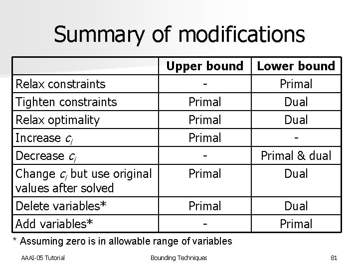
Summary of modifications Upper bound Relax constraints Tighten constraints Primal Relax optimality Primal Increase ci Primal Decrease ci Change ci but use original Primal values after solved Delete variables* Primal Add variables* - Lower bound Primal Dual Primal & dual Dual Primal * Assuming zero is in allowable range of variables AAAI-05 Tutorial Bounding Techniques 81

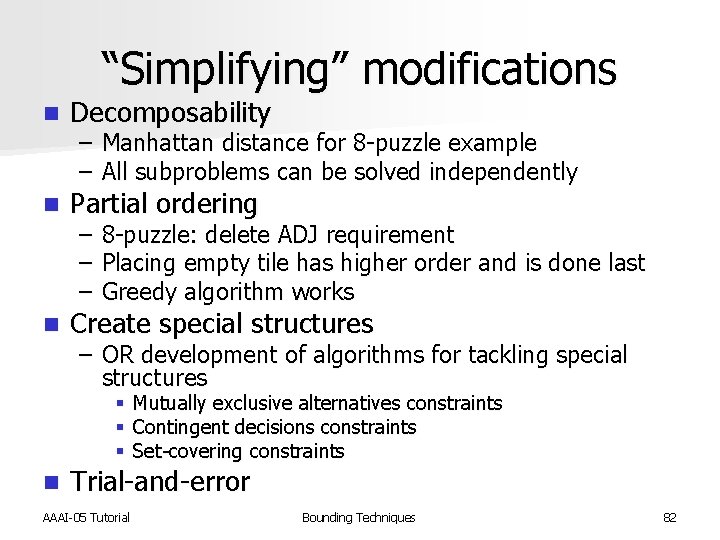
“Simplifying” modifications n Decomposability n Partial ordering n Create special structures – Manhattan distance for 8 -puzzle example – All subproblems can be solved independently – – – 8 -puzzle: delete ADJ requirement Placing empty tile has higher order and is done last Greedy algorithm works – OR development of algorithms for tackling special structures § Mutually exclusive alternatives constraints § Contingent decisions constraints § Set-covering constraints n Trial-and-error AAAI-05 Tutorial Bounding Techniques 82

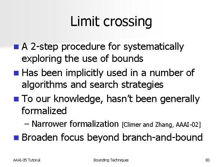
Limit crossing n A 2 -step procedure for systematically exploring the use of bounds n Has been implicitly used in a number of algorithms and search strategies n To our knowledge, hasn’t been generally formalized – Narrower formalization [Climer and Zhang, AAAI-02] n Broaden focus beyond branch-and-bound AAAI-05 Tutorial Bounding Techniques 83

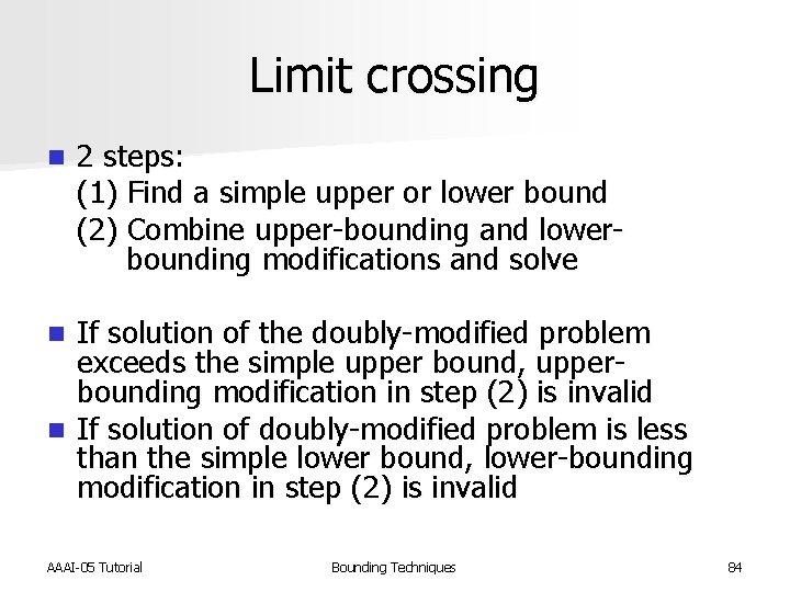
Limit crossing n 2 steps: (1) Find a simple upper or lower bound (2) Combine upper-bounding and lower- bounding modifications and solve If solution of the doubly-modified problem exceeds the simple upper bound, upperbounding modification in step (2) is invalid n If solution of doubly-modified problem is less than the simple lower bound, lower-bounding modification in step (2) is invalid n AAAI-05 Tutorial Bounding Techniques 84

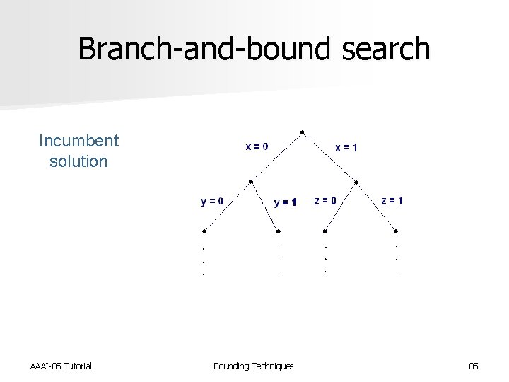
Branch-and-bound search Incumbent solution AAAI-05 Tutorial Bounding Techniques 85

Limit crossing n Find a simple upper or lower bound that is tight n Systematically apply modifications to produce doubly-modified problems – Either modification can be difficult to solve – Only need the combination of the two modifications to be relatively easy n May produce novel search strategies AAAI-05 Tutorial Bounding Techniques 86

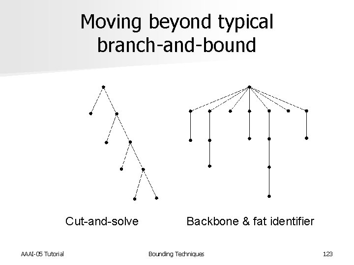
Limit crossing search strategies n Cut-and-solve [Climer and Zhang, AIJ, to appear] – An iterative search strategy – Useful for combinatorial optimization problems n Backbone and fat identifier [Climer and Zhang, AAAI-02] – Used to identify characteristic variables AAAI-05 Tutorial Bounding Techniques 87

Cut-and-solve Iterative search strategy called cut-and-solve n For each iteration: n – Step 1: A chunk of the solution space is cut away and solved, providing incumbent solutions – Step 2: A relaxed solution is found for remaining solution space n Iterate until relaxed solution is greater than or equal to incumbent AAAI-05 Tutorial Bounding Techniques 88

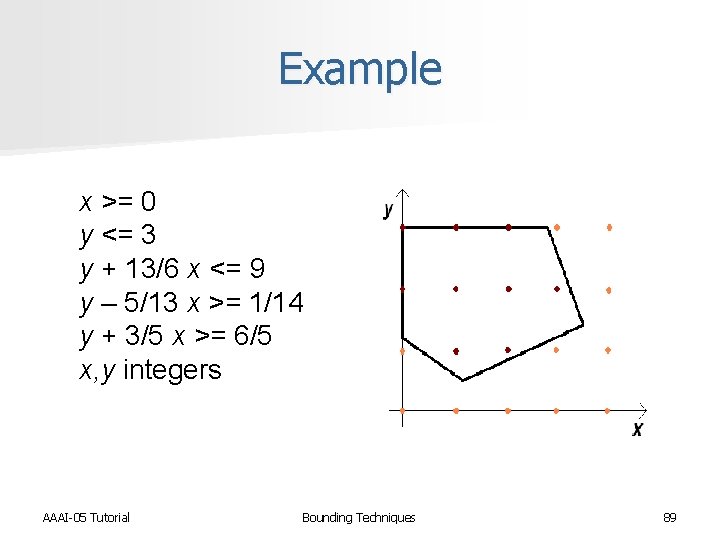
Example x >= 0 y <= 3 y + 13/6 x <= 9 y – 5/13 x >= 1/14 y + 3/5 x >= 6/5 x, y integers AAAI-05 Tutorial Bounding Techniques 89

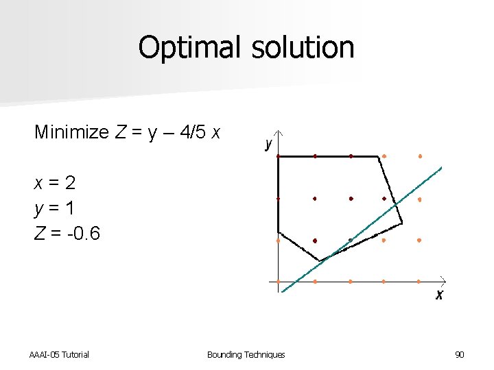
Optimal solution Minimize Z = y – 4/5 x x = 2 y = 1 Z = -0. 6 AAAI-05 Tutorial Bounding Techniques 90

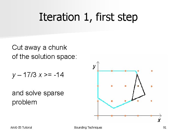
Iteration 1, first step Cut away a chunk of the solution space: y – 17/3 x >= -14 and solve sparse problem AAAI-05 Tutorial Bounding Techniques 91

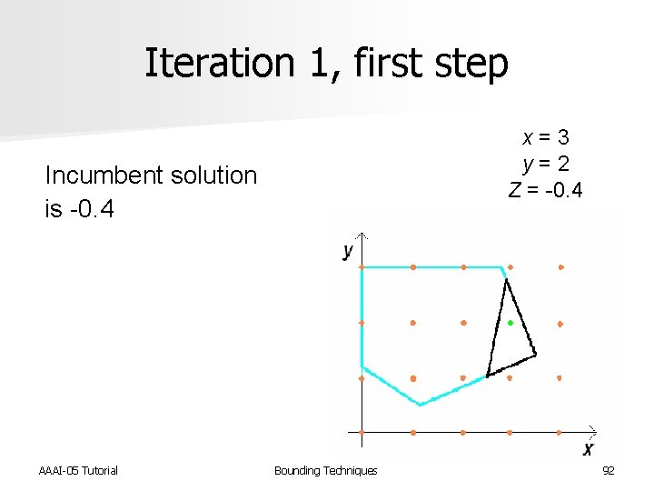
Iteration 1, first step x = 3 y = 2 Z = -0. 4 Incumbent solution is -0. 4 AAAI-05 Tutorial Bounding Techniques 92

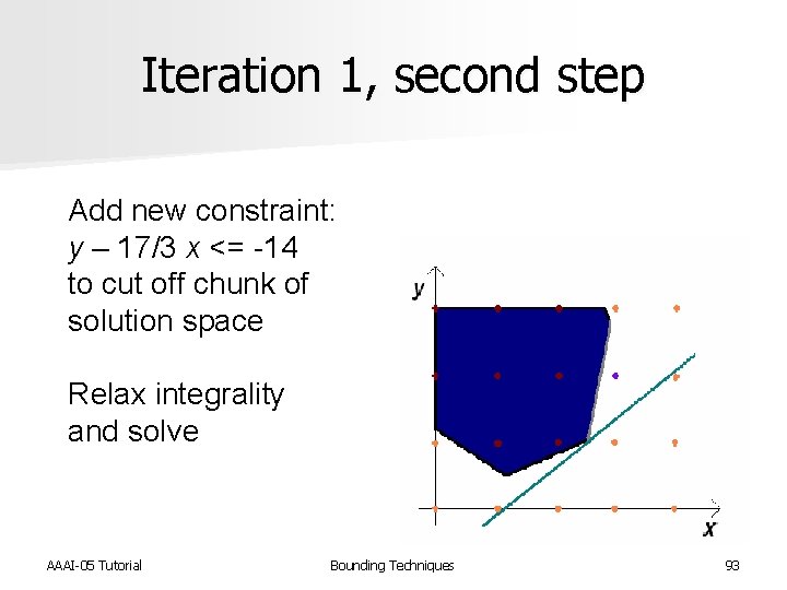
Iteration 1, second step Add new constraint: y – 17/3 x <= -14 to cut off chunk of solution space Relax integrality and solve AAAI-05 Tutorial Bounding Techniques 93

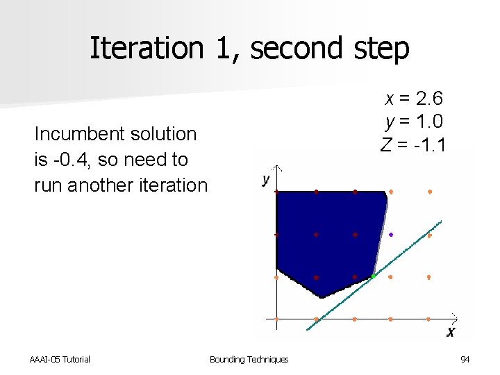
Iteration 1, second step x = 2. 6 y = 1. 0 Z = -1. 1 Incumbent solution is -0. 4, so need to run another iteration AAAI-05 Tutorial Bounding Techniques 94

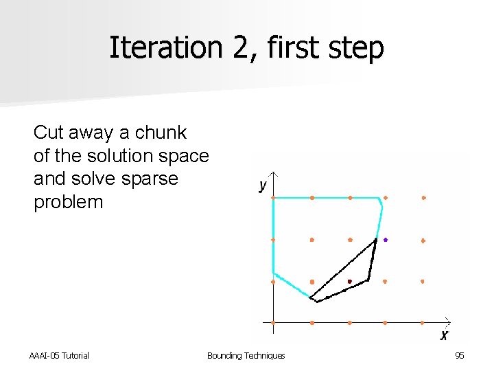
Iteration 2, first step Cut away a chunk of the solution space and solve sparse problem AAAI-05 Tutorial Bounding Techniques 95

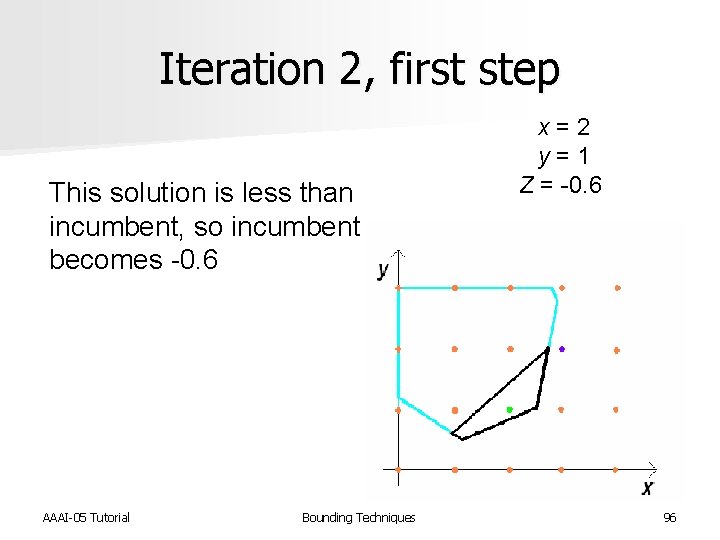
Iteration 2, first step This solution is less than incumbent, so incumbent becomes -0. 6 AAAI-05 Tutorial Bounding Techniques x = 2 y = 1 Z = -0. 6 96

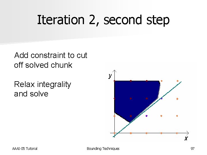
Iteration 2, second step Add constraint to cut off solved chunk Relax integrality and solve AAAI-05 Tutorial Bounding Techniques 97

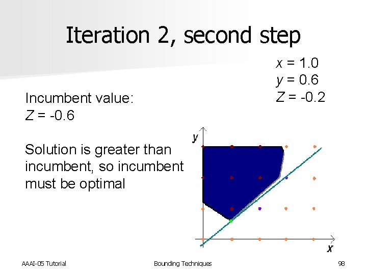
Iteration 2, second step x = 1. 0 y = 0. 6 Z = -0. 2 Incumbent value: Z = -0. 6 Solution is greater than incumbent, so incumbent must be optimal AAAI-05 Tutorial Bounding Techniques 98

Cut-and-solve properties n Minimal memory requirements – Keep new constraints and incumbent solution from one iteration to the next n No subtrees in which to get lost n Piercing cuts should try to capture optimal solutions n Different from conventional cutting planes – Remove solutions from original problem AAAI-05 Tutorial Bounding Techniques 99

Cut-and-solve n Same as two steps of limit crossing – Small chunk is solved to provide simple upper bound – Doubly-modified problem § Added piercing cuts are upper-bounding modifications § Relaxation is lower-bounding modification n Unusual upper-bounding modification – Results in search path instead of search tree AAAI-05 Tutorial Bounding Techniques 100

Cut-and-solve n A general technique for determining piercing cuts for binary IPs – Relax integrality and solve LP – LP yields reduced costs § a lower bound on the increase of the solution if variable forced into LP solution – Let S = set of k variables with the smallest reduced costs – Find optimal solution for set S – Add piercing cut: sum of variables not in S >= 1 n Custom piercing cuts tailored to particular problem may work better AAAI-05 Tutorial Bounding Techniques 101

Cut-and-solve n We used general technique for ATSP [AIJ, to appear] – Piercing cut added: sum of variables in S <= n – 1 – Same cut but less variables in constraint n Very good results for difficult instances – Real-world instances with structural characteristics n Results for easy problems not as impressive AAAI-05 Tutorial Bounding Techniques 102

Backbone and fat identifier n Backbones are variables that appear in every optimal solution n Fat variables don’t appear in any optimal solution n Useful for – Enumerating all optimal solutions – Identifying critical components – Identifying wasted components AAAI-05 Tutorial Bounding Techniques 103

Backbone and fat identifier Find a simple upper bound n Attempt to identify backbones: n – Force exclusion of each variable – If limits cross, must be a backbone n Attempt to identify fat: – Force inclusion of each variable – If limits cross, must be fat Use problem-specific information to improve results n Example for ATSP [Climer and Zhang, AAAI-02] n AAAI-05 Tutorial Bounding Techniques 104

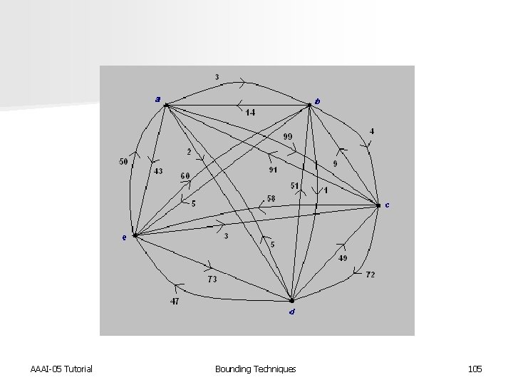
AAAI-05 Tutorial Bounding Techniques 105

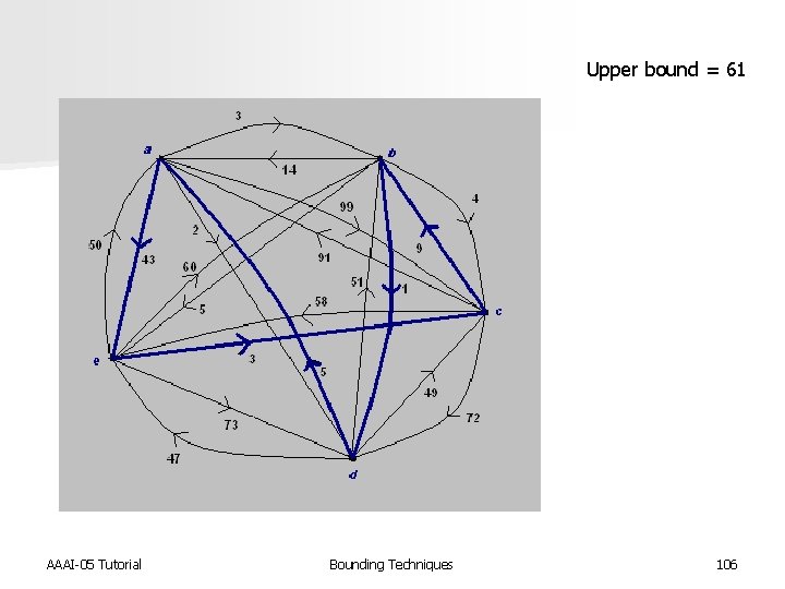
Upper bound = 61 AAAI-05 Tutorial Bounding Techniques 106

Upper bound = 61 AAAI-05 Tutorial Bounding Techniques Lower bound = 24 107

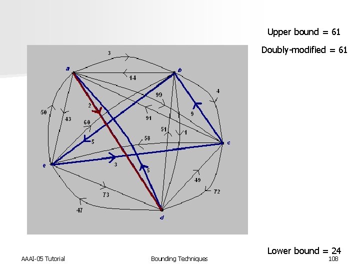
Upper bound = 61 Doubly-modified = 61 AAAI-05 Tutorial Bounding Techniques Lower bound = 24 108

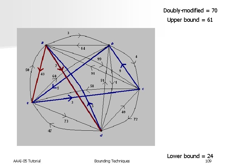
Doubly-modified = 70 Upper bound = 61 AAAI-05 Tutorial Bounding Techniques Lower bound = 24 109

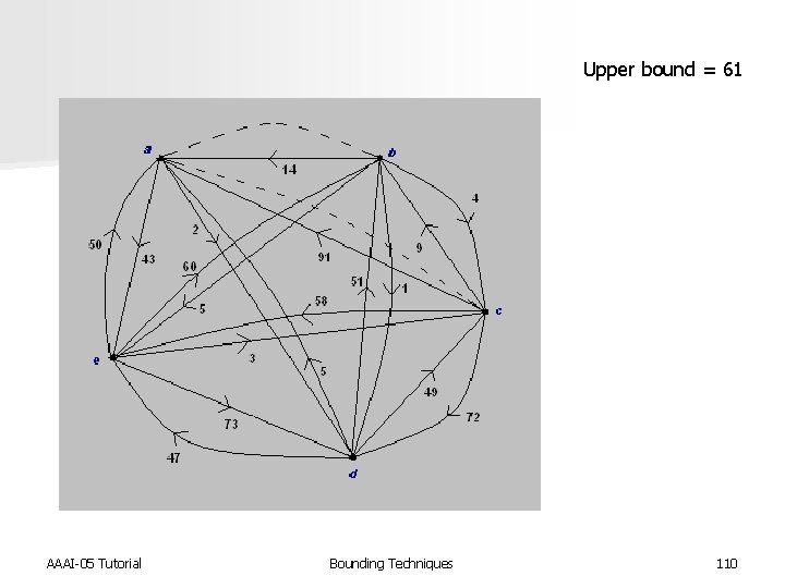
Upper bound = 61 AAAI-05 Tutorial Bounding Techniques 110

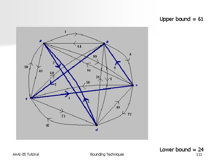
Upper bound = 61 AAAI-05 Tutorial Bounding Techniques Lower bound = 24 111

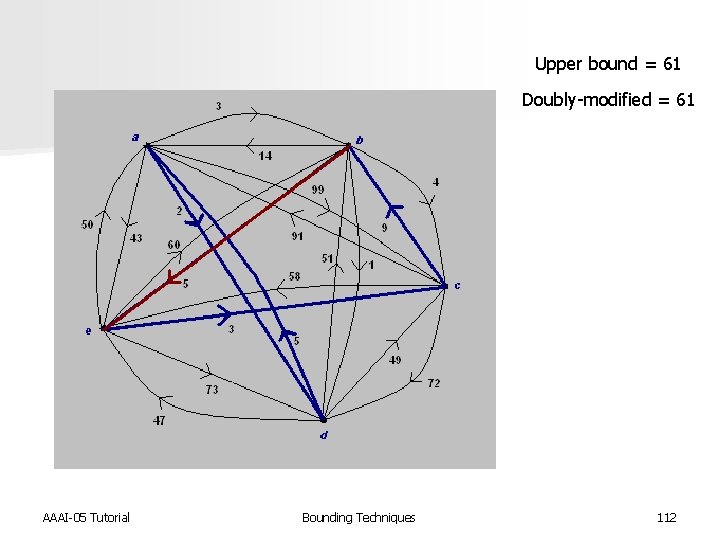
Upper bound = 61 Doubly-modified = 61 AAAI-05 Tutorial Bounding Techniques 112

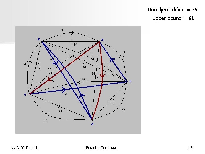
Doubly-modified = 75 Upper bound = 61 AAAI-05 Tutorial Bounding Techniques 113

Upper bound = 61 AAAI-05 Tutorial Bounding Techniques 114

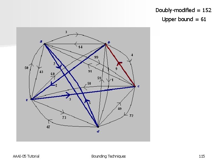
Doubly-modified = 152 Upper bound = 61 AAAI-05 Tutorial Bounding Techniques 115

Upper bound = 61 AAAI-05 Tutorial Bounding Techniques 116

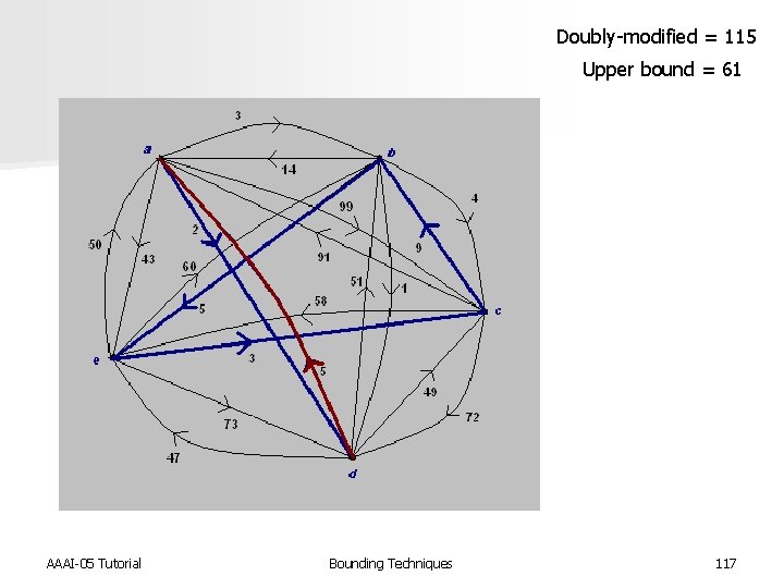
Doubly-modified = 115 Upper bound = 61 AAAI-05 Tutorial Bounding Techniques 117

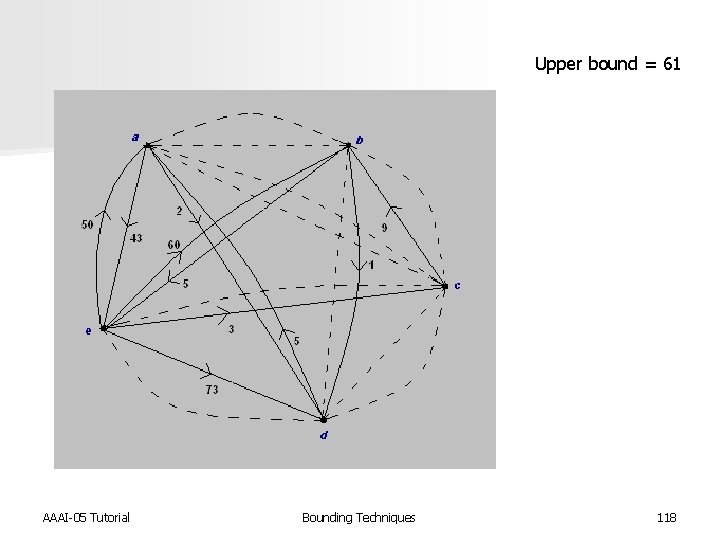
Upper bound = 61 AAAI-05 Tutorial Bounding Techniques 118

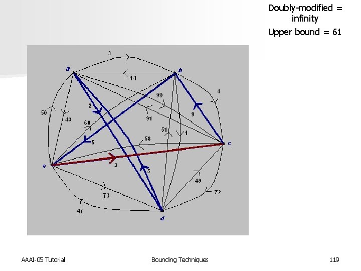
Doubly-modified = infinity Upper bound = 61 AAAI-05 Tutorial Bounding Techniques 119

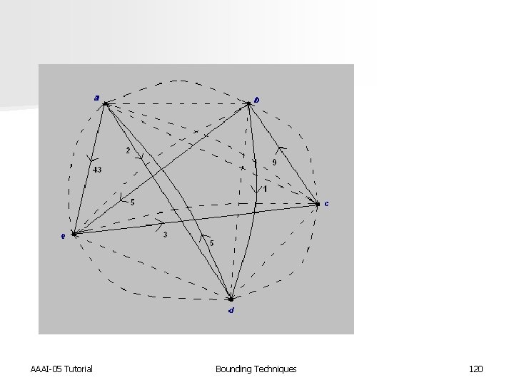
AAAI-05 Tutorial Bounding Techniques 120

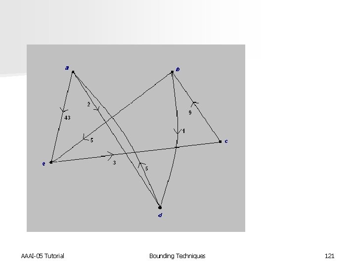
AAAI-05 Tutorial Bounding Techniques 121

Results Used AP lower bound [Climer and Zhang, AAAI-02] Random ATSP graphs with cost range equal to number of cities n Found close to half of the backbone arcs and 99% of the fat arcs n Time savings when finding all solutions: n n – 20% for smaller instances – 75% for larger instances n Found very few backbones and fat for real-world problems as this lower bound is not tight – Implementing with tighter lower bound AAAI-05 Tutorial Bounding Techniques 122

Moving beyond typical branch-and-bound Cut-and-solve AAAI-05 Tutorial Backbone & fat identifier Bounding Techniques 123

Future directions n Forecasting effective bounding modifications – Automatically identifying “easy” doubly-modified problems – Tightness of modifications Systematic exploration of IPs n Other domains n – – – Quadratic programs Constraint programming Explore modifications of every facet of problem definition AAAI-05 Tutorial Bounding Techniques 124

Take-home message The use of bounds is a powerful technique for solving difficult problems n It has been shown that a systematic approach to finding lower bounds can produce useful heuristics that are not easily discovered n Systematically using the 2 -step limit crossing procedure coupled with a clear vision of all potential problem modifications can yield novel search strategies that exploit bounds n AAAI-05 Tutorial Bounding Techniques 125

Questions? AAAI-05 Tutorial Bounding Techniques 126

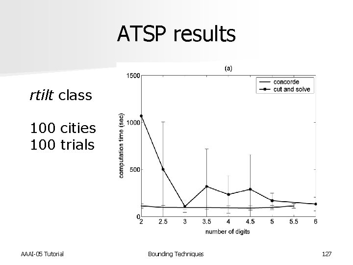
ATSP results rtilt class 100 cities 100 trials AAAI-05 Tutorial Bounding Techniques 127

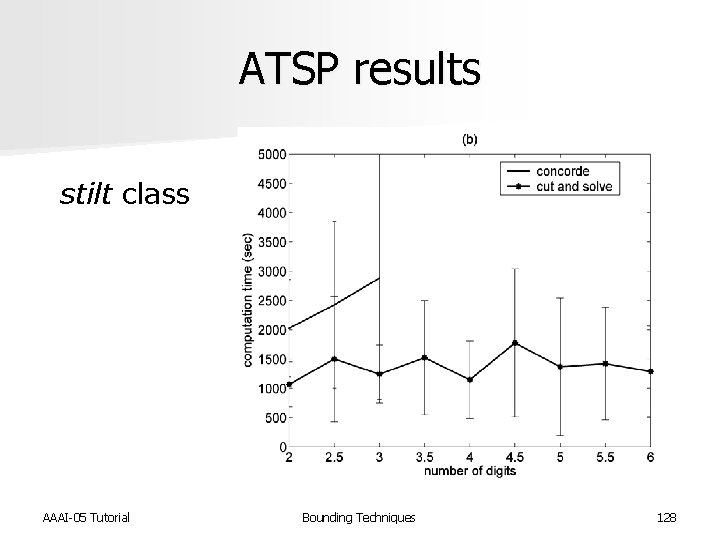
ATSP results stilt class AAAI-05 Tutorial Bounding Techniques 128

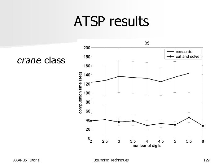
ATSP results crane class AAAI-05 Tutorial Bounding Techniques 129

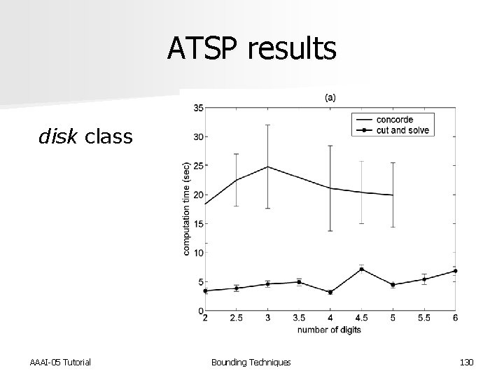
ATSP results disk class AAAI-05 Tutorial Bounding Techniques 130

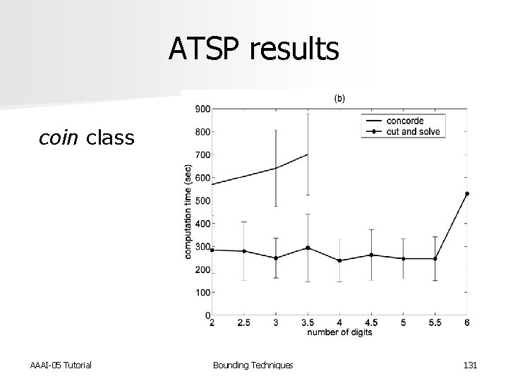
ATSP results coin class AAAI-05 Tutorial Bounding Techniques 131

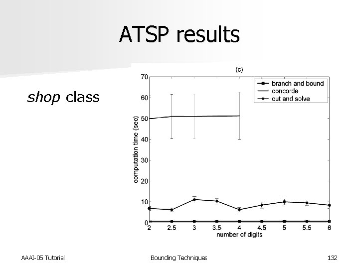
ATSP results shop class AAAI-05 Tutorial Bounding Techniques 132