System of Linear Equations System of Linear Equations

System of Linear Equations

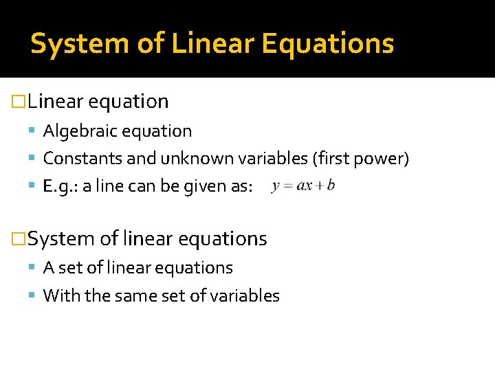
System of Linear Equations �Linear equation Algebraic equation Constants and unknown variables (first power) E. g. : a line can be given as: �System of linear equations A set of linear equations With the same set of variables

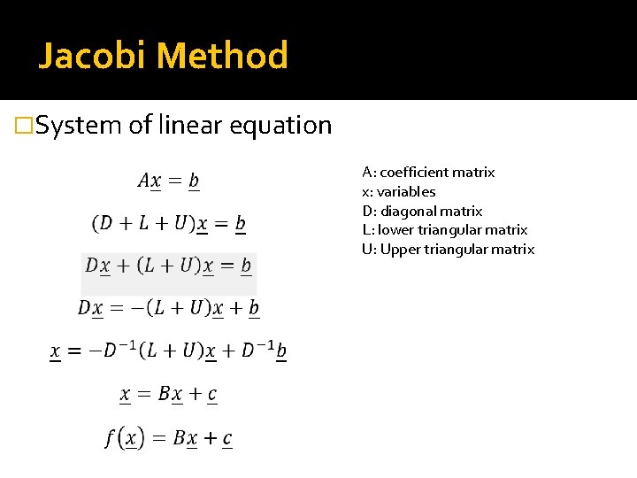
Jacobi Method �System of linear equation A: coefficient matrix x: variables D: diagonal matrix L: lower triangular matrix U: Upper triangular matrix

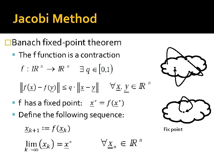
Jacobi Method �Banach fixed-point theorem The f function is a contraction f has a fixed point: Define the following sequence: Fix point

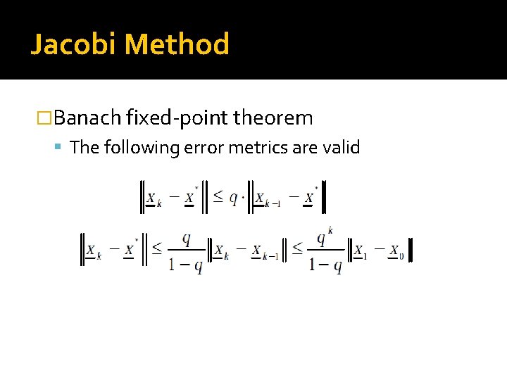
Jacobi Method �Banach fixed-point theorem The following error metrics are valid

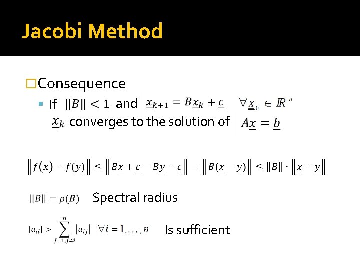
Jacobi Method �Consequence If and converges to the solution of Spectral radius Is sufficient

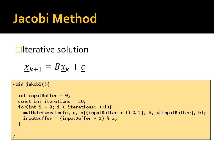
Jacobi Method �Iterative solution void jakobi(){. . . int input. Buffer = 0; const int iterations = 20; for(int i = 0; i < iterations; ++i){ mul. Matrix. Vector(n, n, x[(input. Buffer + 1) % 2], A, x[input. Buffer], b); input. Buffer = (input. Buffer + 1) % 2; }. . . }

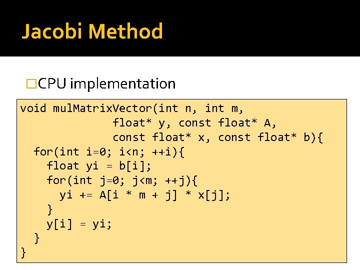
Jacobi Method �CPU implementation void mul. Matrix. Vector(int n, int m, float* y, const float* A, const float* x, const float* b){ for(int i=0; i<n; ++i){ float yi = b[i]; for(int j=0; j<m; ++j){ yi += A[i * m + j] * x[j]; } y[i] = yi; } }

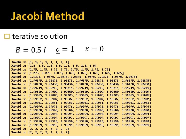
Jacobi Method �Iterative solution Jakobi Jakobi Jakobi Jakobi Jakobi x: x: x: x: x: [1, 1, 1] [1. 5, 1. 5] [1. 75, 1. 75] [1. 875, 1. 875] [1. 9375, 1. 9375] [1. 96875, 1. 96875] [1. 98438, 1. 98438] [1. 99219, 1. 99219] [1. 99609, 1. 99609] [1. 99805, 1. 99805] [1. 99902, 1. 99902] [1. 99951, 1. 99951] [1. 99976, 1. 99976] [1. 99988, 1. 99988] [1. 99994, 1. 99994] [1. 99997, 1. 99997] [1. 99998, 1. 99998] [1. 99999, 1. 99999] [2, 2, 2, 2, 2]

Matrix Vector Multiplication �Parallelization Assign threads to the result elements ▪ Gather: each thread summarizes the contribution of each input element Assign threads to the input elements ▪ Scatter: each thread calculates the contribution of an input element to the output elements ▪ Synchronization needed!

Matrix Vector Multiplication �Gather The result is a vector with N elements The size of the job is N Each thread calculates one element in the result vector using one row of the matrix and the input vector Over indexing shall be checked!

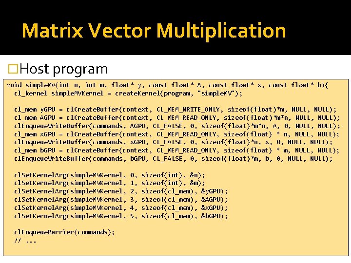
Matrix Vector Multiplication �Host program void simple. MV(int n, int m, float* y, const float* A, const float* x, const float* b){ cl_kernel simple. MVKernel = create. Kernel(program, "simple. MV"); cl_mem y. GPU = cl. Create. Buffer(context, CL_MEM_WRITE_ONLY, sizeof(float)*m, NULL); cl_mem AGPU = cl. Create. Buffer(context, CL_MEM_READ_ONLY, sizeof(float)*m*n, NULL); cl. Enqueue. Write. Buffer(commands, AGPU, CL_FALSE, 0, sizeof(float)*m*n, A, 0, NULL); cl_mem x. GPU = cl. Create. Buffer(context, CL_MEM_READ_ONLY, sizeof(float) * n, NULL); cl. Enqueue. Write. Buffer(commands, x. GPU, CL_FALSE, 0, sizeof(float)*n, x, 0, NULL); cl_mem b. GPU = cl. Create. Buffer(context, CL_MEM_READ_ONLY, sizeof(float) * m, NULL); cl. Enqueue. Write. Buffer(commands, b. GPU, CL_FALSE, 0, sizeof(float)*m, b, 0, NULL); cl. Set. Kernel. Arg(simple. MVKernel, cl. Enqueue. Barrier(commands); //. . . 0, 1, 2, 3, 4, 5, sizeof(int), &n); sizeof(int), &m); sizeof(cl_mem), &y. GPU); sizeof(cl_mem), &AGPU); sizeof(cl_mem), &x. GPU); sizeof(cl_mem), &b. GPU);

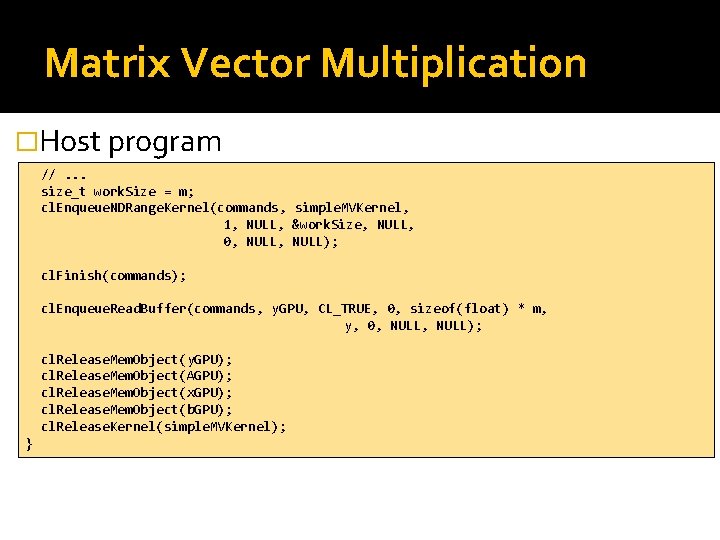
Matrix Vector Multiplication �Host program //. . . size_t work. Size = m; cl. Enqueue. NDRange. Kernel(commands, simple. MVKernel, 1, NULL, &work. Size, NULL, 0, NULL); cl. Finish(commands); cl. Enqueue. Read. Buffer(commands, y. GPU, CL_TRUE, 0, sizeof(float) * m, y, 0, NULL); cl. Release. Mem. Object(y. GPU); cl. Release. Mem. Object(AGPU); cl. Release. Mem. Object(x. GPU); cl. Release. Mem. Object(b. GPU); cl. Release. Kernel(simple. MVKernel); }

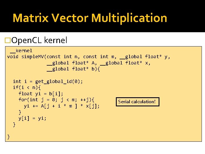
Matrix Vector Multiplication �Open. CL kernel __kernel void simple. MV(const int n, const int m, __global float* y, __global float* A, __global float* x, __global float* b){ int i = get_global_id(0); if(i < n){ float yi = b[i]; for(int j = 0; j < m; ++j){ yi += A[j + i * m ] * x[j]; } y[i] = yi; } } Serial calculation!

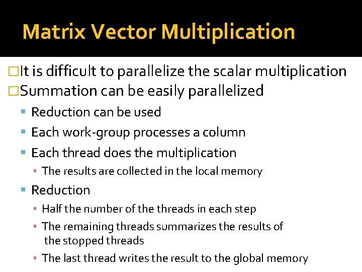
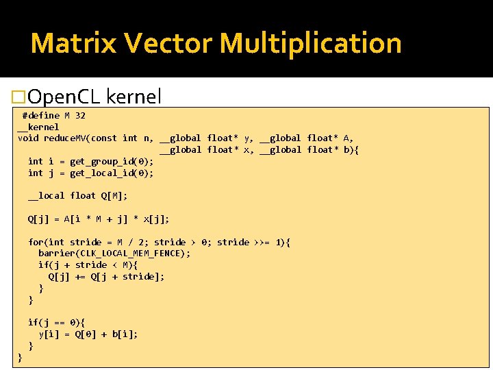
Matrix Vector Multiplication �It is difficult to parallelize the scalar multiplication �Summation can be easily parallelized Reduction can be used Each work-group processes a column Each thread does the multiplication ▪ The results are collected in the local memory Reduction ▪ Half the number of the threads in each step ▪ The remaining threads summarizes the results of the stopped threads ▪ The last thread writes the result to the global memory

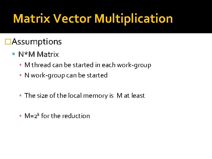
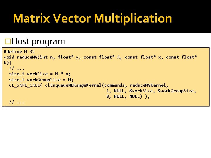
Matrix Vector Multiplication �Assumptions N*M Matrix ▪ M thread can be started in each work-group ▪ N work-group can be started ▪ The size of the local memory is M at least ▪ M=2 k for the reduction

Matrix Vector Multiplication �Host program #define M 32 void reduce. MV(int n, float* y, const float* A, const float* x, const float* b){ //. . . size_t work. Size = M * n; size_t work. Group. Size = M; CL_SAFE_CALL( cl. Enqueue. NDRange. Kernel(commands, reduce. MVKernel, 1, NULL, &work. Size, &work. Group. Size, 0, NULL) ); //. . . }

Matrix Vector Multiplication �Open. CL kernel #define M 32 __kernel void reduce. MV(const int n, __global float* y, __global float* A, __global float* x, __global float* b){ int i = get_group_id(0); int j = get_local_id(0); __local float Q[M]; Q[j] = A[i * M + j] * x[j]; for(int stride = M / 2; stride > 0; stride >>= 1){ barrier(CLK_LOCAL_MEM_FENCE); if(j + stride < M){ Q[j] += Q[j + stride]; } } if(j == 0){ y[i] = Q[0] + b[i]; } }

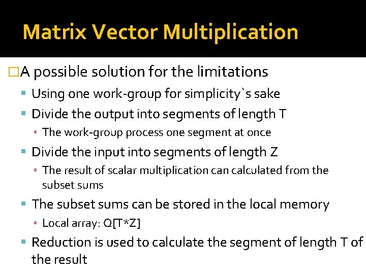
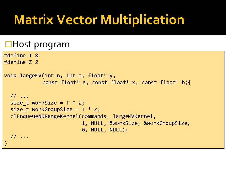
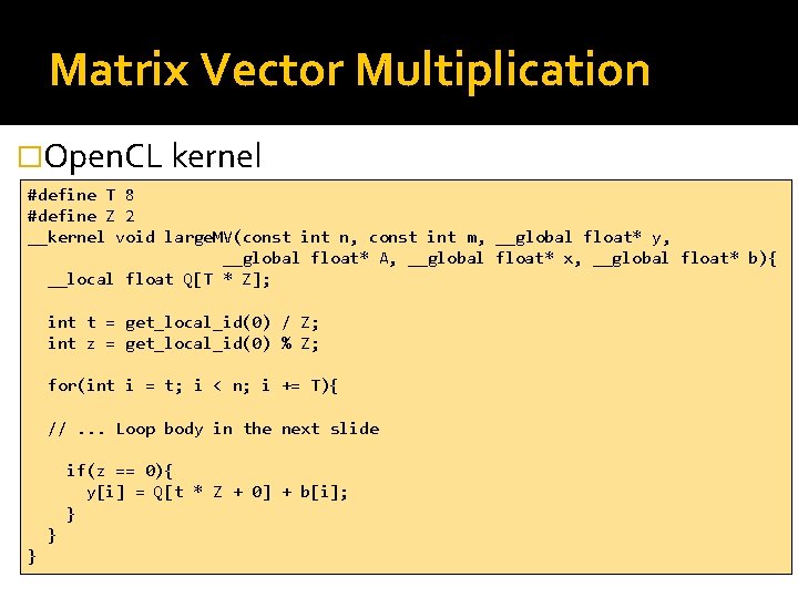
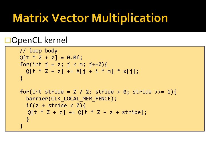
Matrix Vector Multiplication �A possible solution for the limitations Using one work-group for simplicity`s sake Divide the output into segments of length T ▪ The work-group process one segment at once Divide the input into segments of length Z ▪ The result of scalar multiplication calculated from the subset sums The subset sums can be stored in the local memory ▪ Local array: Q[T*Z] Reduction is used to calculate the segment of length T of the result

Matrix Vector Multiplication �Host program #define T 8 #define Z 2 void large. MV(int n, int m, float* y, const float* A, const float* x, const float* b){ //. . . size_t work. Size = T * Z; size_t work. Group. Size = T * Z; cl. Enqueue. NDRange. Kernel(commands, large. MVKernel, 1, NULL, &work. Size, &work. Group. Size, 0, NULL); //. . . }

Matrix Vector Multiplication �Open. CL kernel #define T 8 #define Z 2 __kernel void large. MV(const int n, const int m, __global float* y, __global float* A, __global float* x, __global float* b){ __local float Q[T * Z]; int t = get_local_id(0) / Z; int z = get_local_id(0) % Z; for(int i = t; i < n; i += T){ //. . . Loop body in the next slide if(z == 0){ y[i] = Q[t * Z + 0] + b[i]; } } }

Matrix Vector Multiplication �Open. CL kernel // loop Q[t * Z for(int Q[t * } body + z] = 0. 0 f; j = z; j < m; j+=Z){ Z + z] += A[j + i * m] * x[j]; for(int stride = Z / 2; stride > 0; stride >>= 1){ barrier(CLK_LOCAL_MEM_FENCE); if(z + stride < Z){ Q[t * Z + z] += Q[t * Z + z + stride]; } }

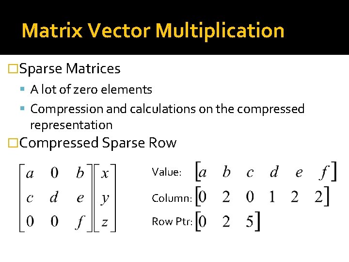
Matrix Vector Multiplication �Sparse Matrices A lot of zero elements Compression and calculations on the compressed representation �Compressed Sparse Row Value: Column: Row Ptr:

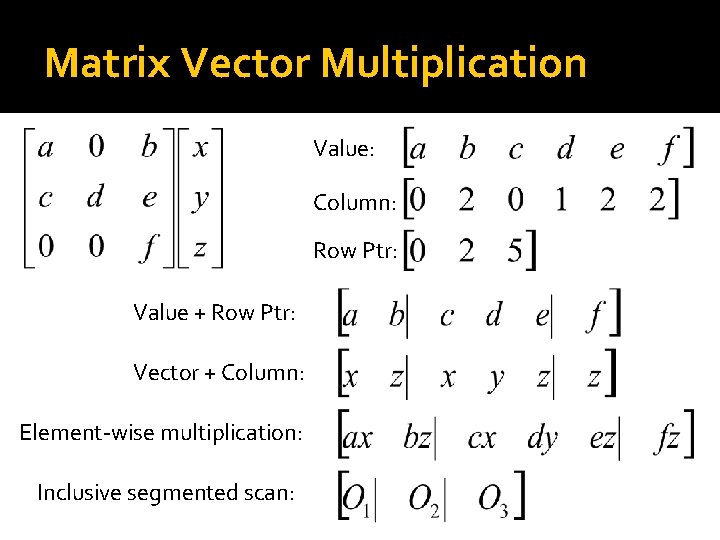
Matrix Vector Multiplication Value: Column: Row Ptr: Value + Row Ptr: Vector + Column: Element-wise multiplication: Inclusive segmented scan:

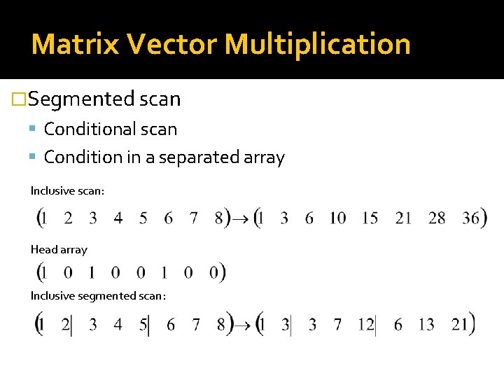
Matrix Vector Multiplication �Segmented scan Conditional scan Condition in a separated array Inclusive scan: Head array Inclusive segmented scan:

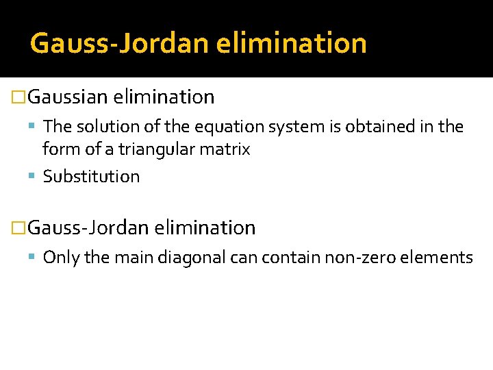
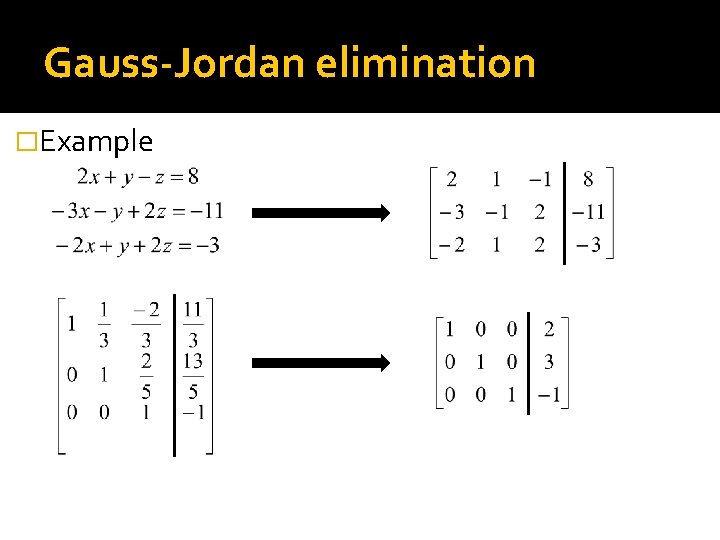
Gauss-Jordan elimination �Gaussian elimination The solution of the equation system is obtained in the form of a triangular matrix Substitution �Gauss-Jordan elimination Only the main diagonal can contain non-zero elements

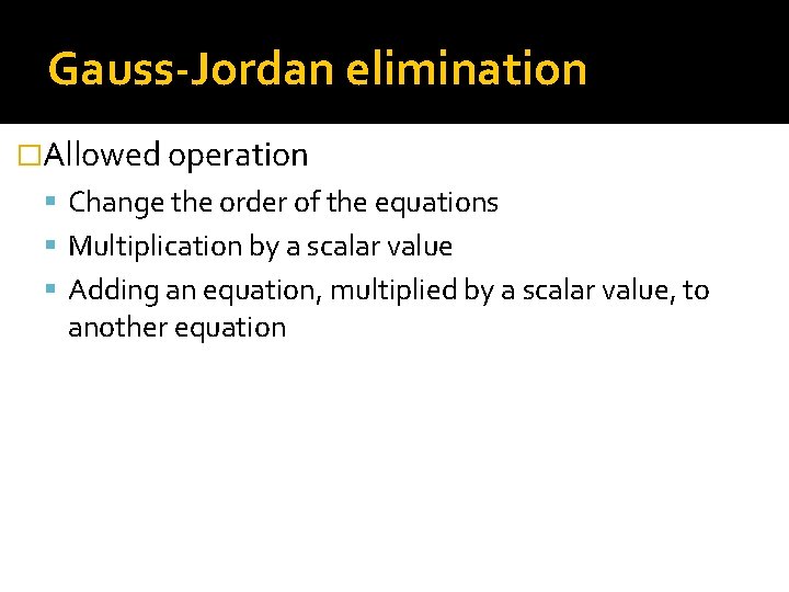
Gauss-Jordan elimination �Allowed operation Change the order of the equations Multiplication by a scalar value Adding an equation, multiplied by a scalar value, to another equation

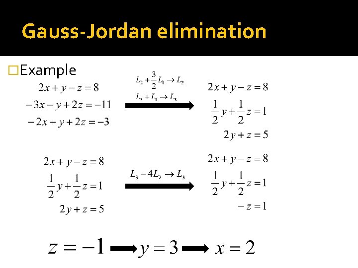
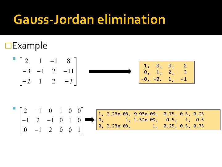
Gauss-Jordan elimination �Example

Gauss-Jordan elimination �Example

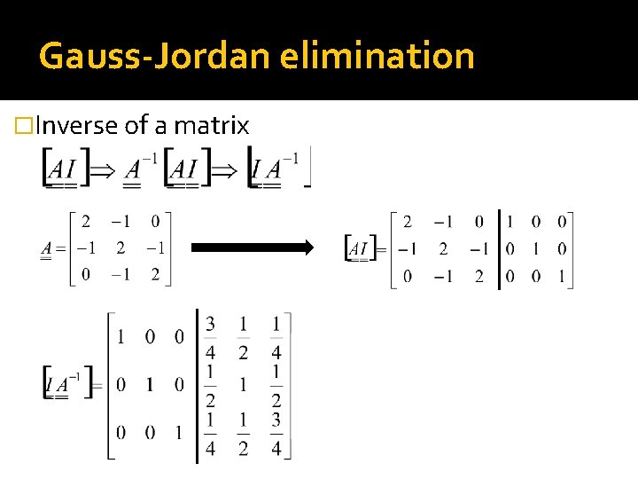
Gauss-Jordan elimination �Inverse of a matrix

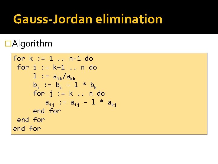
Gauss-Jordan elimination �Algorithm for k : = 1. . n-1 do for i : = k+1. . n do l : = aik/akk bi : = bi – l * bk for j : = k. . n do aij : = aij – l * akj end for

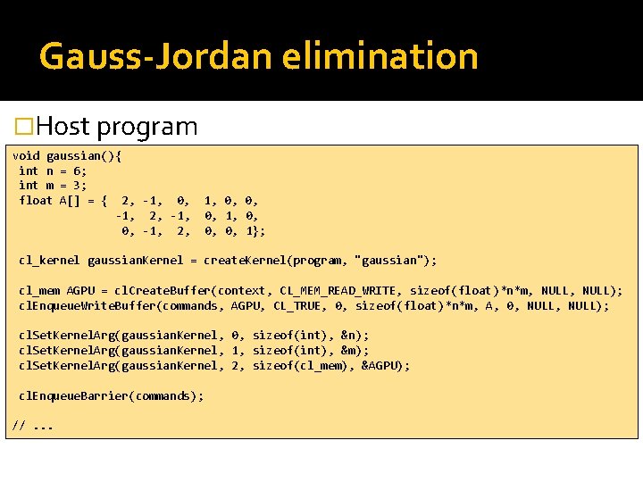
Gauss-Jordan elimination �Host program void gaussian(){ int n = 6; int m = 3; float A[] = { 2, -1, 0, -1, 2, 1, 0, 0, 0, 1}; cl_kernel gaussian. Kernel = create. Kernel(program, "gaussian"); cl_mem AGPU = cl. Create. Buffer(context, CL_MEM_READ_WRITE, sizeof(float)*n*m, NULL); cl. Enqueue. Write. Buffer(commands, AGPU, CL_TRUE, 0, sizeof(float)*n*m, A, 0, NULL); cl. Set. Kernel. Arg(gaussian. Kernel, 0, sizeof(int), &n); cl. Set. Kernel. Arg(gaussian. Kernel, 1, sizeof(int), &m); cl. Set. Kernel. Arg(gaussian. Kernel, 2, sizeof(cl_mem), &AGPU); cl. Enqueue. Barrier(commands); //. . .

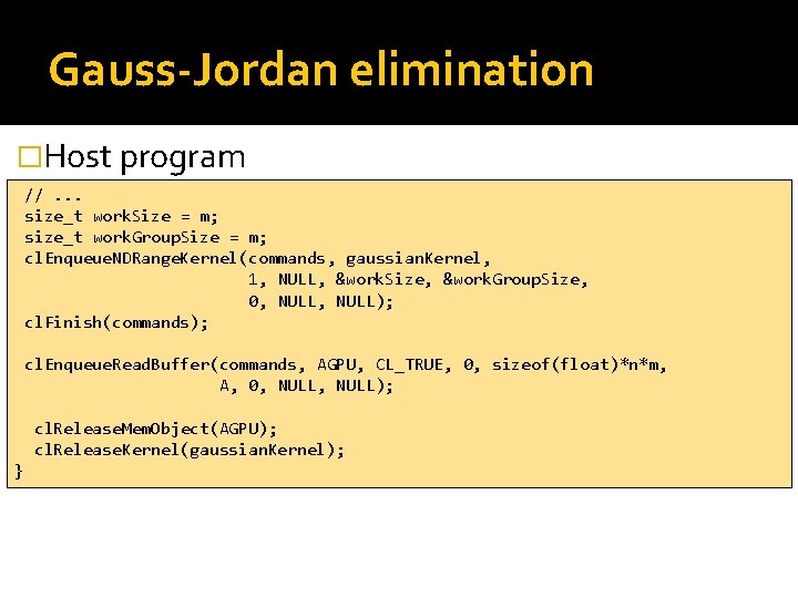
Gauss-Jordan elimination �Host program //. . . size_t work. Size = m; size_t work. Group. Size = m; cl. Enqueue. NDRange. Kernel(commands, gaussian. Kernel, 1, NULL, &work. Size, &work. Group. Size, 0, NULL); cl. Finish(commands); cl. Enqueue. Read. Buffer(commands, AGPU, CL_TRUE, 0, sizeof(float)*n*m, A, 0, NULL); cl. Release. Mem. Object(AGPU); cl. Release. Kernel(gaussian. Kernel); }

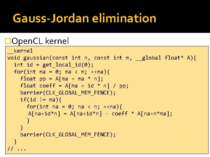
Gauss-Jordan elimination �Open. CL kernel __kernel void gaussian(const int n, const int m, __global float* A){ int id = get_local_id(0); for(int ma = 0; ma < m; ++ma){ float pp = A[ma + ma * n]; float coeff = A[ma + id * n] / pp; barrier(CLK_GLOBAL_MEM_FENCE); if(id != ma){ for(int na = 0; na < n; ++na){ A[na+id*n] = A[na+id*n] - coeff * A[na+n*ma]; } } barrier(CLK_GLOBAL_MEM_FENCE); } //. . .

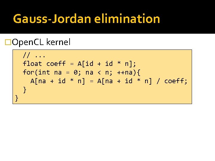
Gauss-Jordan elimination �Open. CL kernel //. . . float coeff = A[id + id * n]; for(int na = 0; na < n; ++na){ A[na + id * n] = A[na + id * n] / coeff; } }

Gauss-Jordan elimination �Example 1, 0, 0, 1, -0, 1, 2. 23 e-08, 9. 93 e-09, 0, 1, 1. 32 e-08, 0, 2. 23 e-08, 1, 0, 0, 1, 2 3 -1 0. 75, 0. 25 0. 5, 1, 0. 5 0. 25, 0. 75