System Modeling and Identification Lecture 1 Dr Ing

System Modeling and Identification Lecture 1 Dr. -Ing. Erwin Sitompul President University http: //zitompul. wordpress. com 2 0 1 5 President University Erwin Sitompul SMI 1/1

System Modeling and Identification Textbook and Syllabus Textbook: “Process Modelling, Identification, and Control”, Jan Mikles, Miroslav Fikar, Springer, 2007. Syllabus: Chapter 1: Introduction Chapter 2: Mathematical Modeling of Processes Chapter 3: Analysis of Process Models Chapter 4: Dynamical Behavior of Processes Chapter 5: Discrete-Time Process Models Chapter 6: Process Identification President University Erwin Sitompul SMI 1/2

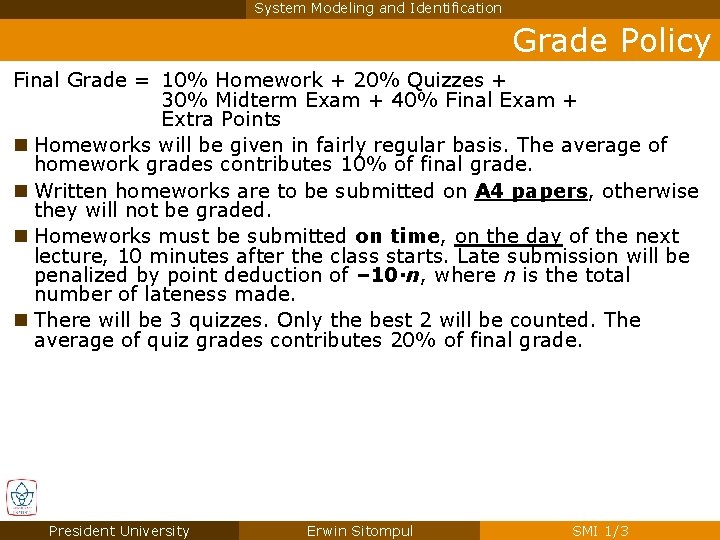
System Modeling and Identification Grade Policy Final Grade = 10% Homework + 20% Quizzes + 30% Midterm Exam + 40% Final Exam + Extra Points n Homeworks will be given in fairly regular basis. The average of homework grades contributes 10% of final grade. n Written homeworks are to be submitted on A 4 papers, otherwise they will not be graded. n Homeworks must be submitted on time, on the day of the next lecture, 10 minutes after the class starts. Late submission will be penalized by point deduction of – 10·n, where n is the total number of lateness made. n There will be 3 quizzes. Only the best 2 will be counted. The average of quiz grades contributes 20% of final grade. President University Erwin Sitompul SMI 1/3

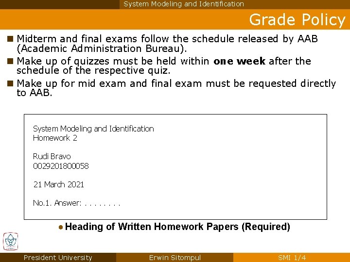
System Modeling and Identification Grade Policy n Midterm and final exams follow the schedule released by AAB (Academic Administration Bureau). n Make up of quizzes must be held within one week after the schedule of the respective quiz. n Make up for mid exam and final exam must be requested directly to AAB. System Modeling and Identification Homework 2 Rudi Bravo 0029201800058 21 March 2021 No. 1. Answer: . . . . ● Heading of Written Homework Papers (Required) President University Erwin Sitompul SMI 1/4

System Modeling and Identification Grade Policy n Extra points will be given if you solve a problem in front of the class. You will earn 1 or 2. n Lecture slides can be copied during class session. It is also available on internet. Please check the course homepage regularly. http: //zitompul. wordpress. com n The use of internet for any purpose during class sessions is strictly forbidden. n You are expected to write a note along the lectures to record your own conclusions or materials which are not covered by the lecture slides. President University Erwin Sitompul SMI 1/5

System Modeling and Identification Chapter 1 Introduction President University Erwin Sitompul SMI 1/6

Chapter 1 Introduction Control is the purposeful influence on an object (process) to ensure the fulfillment of a required objectives. n The objectives can be to satisfy the safety and optimal operation of the technology, the product specifications under constraints of disturbance, process stability, and other technical related matters. n Control systems in the whole consist of technical devices and human factor. Control systems must satisfy: n Disturbance attenuation n Stability guarantee n Optimal process operation President University Erwin Sitompul SMI 1/7

Chapter 1 Introduction Control n There are two main methods of control: n Feedback control, where the information about process output is used to calculate the control (manipulated) signal process output is fed back to process input n Feedforward control, where the effect of control is not compared with the desired result n Practical control experience confirms the importance of assumptions about dynamical behavior of processes. n This behavior is described using mathematical models of processes, which can be constructed from a physical or chemical nature of processes or can be abstract. President University Erwin Sitompul SMI 1/8

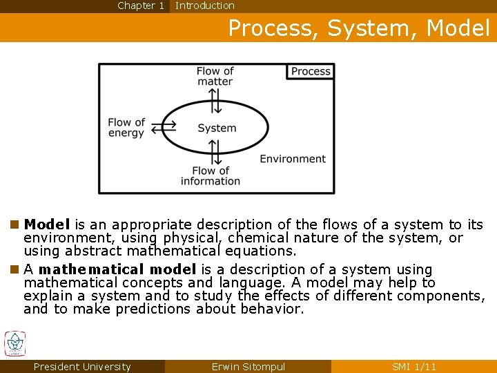
Chapter 1 Introduction Process, System, Model n The purpose of this course is to learn how to model a process, which may have one of these objectives: n Synthesis: Modeling as the fundamentals to influence a process through a controller n Analysis: Modeling as the fundamentals to a deep understanding of the process and further to optimization of the process n Simulation: Modeling as the fundamentals to emulative calculation under a given boundary condition n Process is the entire activities where matter and/or energy are stored, transported, and converted; whereas information is stored, transported, converted, created, or destroyed. n System is a part of a process, which is defined by the user, and has an interconnection with the environment regarding the flow of matter, energy, and information. President University Erwin Sitompul SMI 1/9

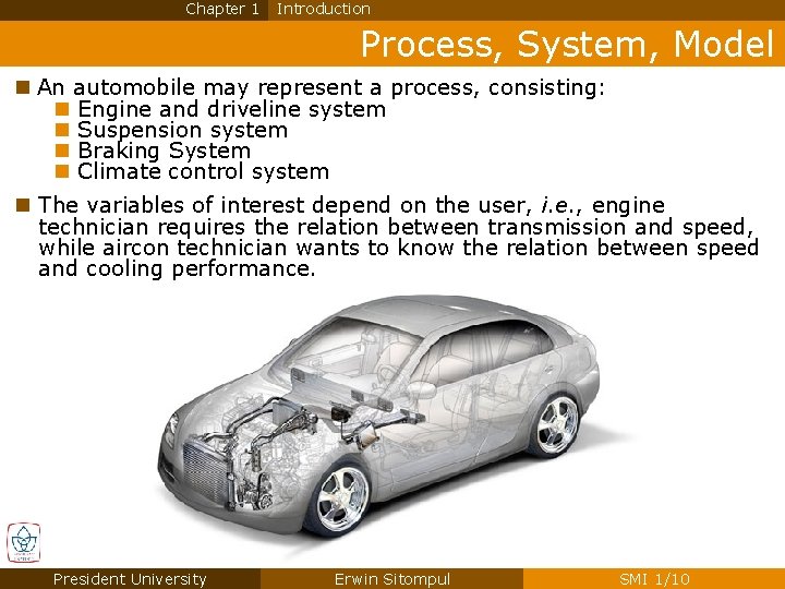
Chapter 1 Introduction Process, System, Model n An automobile may represent a process, consisting: n Engine and driveline system n Suspension system n Braking System n Climate control system n The variables of interest depend on the user, i. e. , engine technician requires the relation between transmission and speed, while aircon technician wants to know the relation between speed and cooling performance. President University Erwin Sitompul SMI 1/10

Chapter 1 Introduction Process, System, Model n Model is an appropriate description of the flows of a system to its environment, using physical, chemical nature of the system, or using abstract mathematical equations. n A mathematical model is a description of a system using mathematical concepts and language. A model may help to explain a system and to study the effects of different components, and to make predictions about behavior. President University Erwin Sitompul SMI 1/11

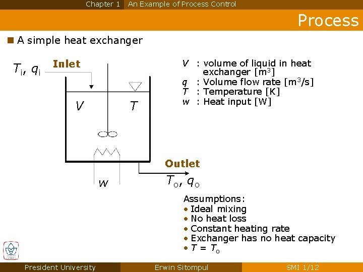
Chapter 1 An Example of Process Control Process n A simple heat exchanger Ti, qi Inlet V T V : volume of liquid in heat exchanger [m 3] q : Volume flow rate [m 3/s] T : Temperature [K] w : Heat input [W] Outlet w T o , qo Assumptions: • Ideal mixing • No heat loss • Constant heating rate • Exchanger has no heat capacity • T = To President University Erwin Sitompul SMI 1/12

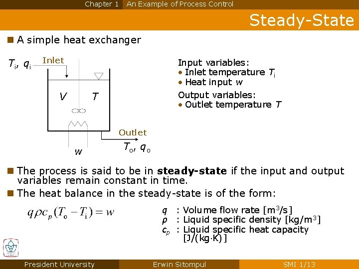
Chapter 1 An Example of Process Control Steady-State n A simple heat exchanger T i , qi Inlet V Input variables: • Inlet temperature Ti • Heat input w Output variables: • Outlet temperature T T Outlet w T o, qo n The process is said to be in steady-state if the input and output variables remain constant in time. n The heat balance in the steady-state is of the form: q : Volume flow rate [m 3/s] ρ : Liquid specific density [kg/m 3] cp : Liquid specific heat capacity [J/(kg K)] President University Erwin Sitompul SMI 1/13

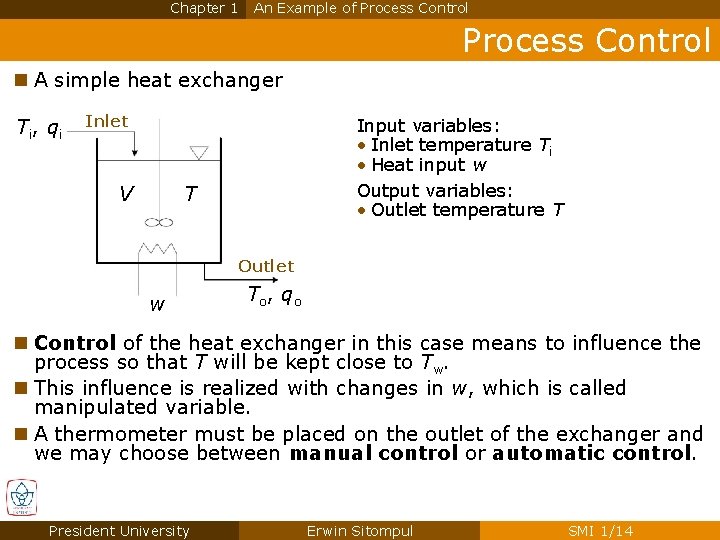
Chapter 1 An Example of Process Control n A simple heat exchanger T i , qi Inlet V Input variables: • Inlet temperature Ti • Heat input w Output variables: • Outlet temperature T T Outlet w T o, qo n Control of the heat exchanger in this case means to influence the process so that T will be kept close to Tw. n This influence is realized with changes in w, which is called manipulated variable. n A thermometer must be placed on the outlet of the exchanger and we may choose between manual control or automatic control. President University Erwin Sitompul SMI 1/14

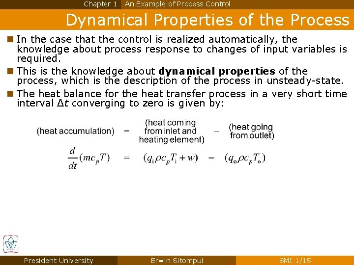
Chapter 1 An Example of Process Control Dynamical Properties of the Process n In the case that the control is realized automatically, the knowledge about process response to changes of input variables is required. n This is the knowledge about dynamical properties of the process, which is the description of the process in unsteady-state. n The heat balance for the heat transfer process in a very short time interval Δt converging to zero is given by: President University Erwin Sitompul SMI 1/15

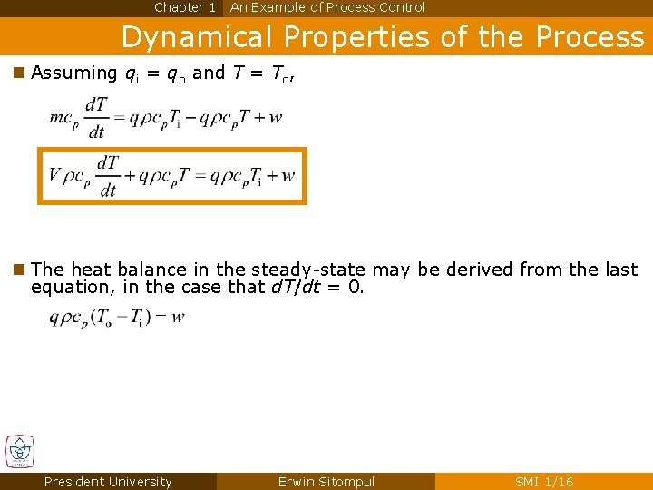
Chapter 1 An Example of Process Control Dynamical Properties of the Process n Assuming qi = qo and T = To, n The heat balance in the steady-state may be derived from the last equation, in the case that d. T/dt = 0. President University Erwin Sitompul SMI 1/16

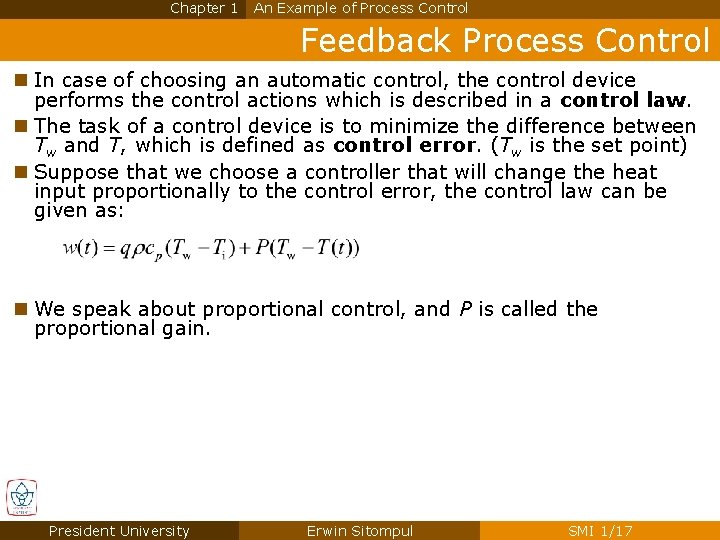
Chapter 1 An Example of Process Control Feedback Process Control n In case of choosing an automatic control, the control device performs the control actions which is described in a control law. n The task of a control device is to minimize the difference between Tw and T, which is defined as control error. (Tw is the set point) n Suppose that we choose a controller that will change the heat input proportionally to the control error, the control law can be given as: n We speak about proportional control, and P is called the proportional gain. President University Erwin Sitompul SMI 1/17

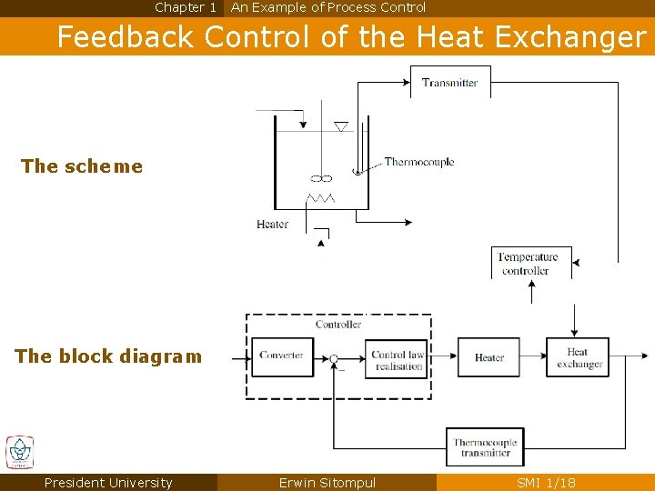
Chapter 1 An Example of Process Control Feedback Control of the Heat Exchanger The scheme The block diagram President University Erwin Sitompul SMI 1/18

System Modeling and Identification Chapter 2 Mathematical Modeling of Processes President University Erwin Sitompul SMI 1/19

Chapter 2 Mathematical Modeling of Processes General Principles of Modeling n A system is expressed through mathematical descriptions. n These descriptions are called “mathematical models. ” n The behavior of the system with regard to certain inputs can be characterized by using the mathematical model. n Mathematical models can be divided into three groups, depending on how they are obtained: n Theoretical model, developed using physical, chemical principles/laws n Empirical model, obtained from mathematical analysis of measurement data of the process/ system or through experience n Empirical-theoretical model, obtained from a combination of theoretical and empirical modeling approach President University Erwin Sitompul SMI 1/20

Chapter 2 Mathematical Modeling of Processes General Principles of Modeling n Theoretical models are derived from the so called “balance equation of conserved quantity” that may include: n Mass balance equation n Energy balance equation n Entropy balance equation n Enthalpy balance equation n Charge balance equation n Heat balance equation n Impulse balance equation n A conserved quantity is a quantity whose total amount is maintained constant and is understood to obey the principle of conservation, which states that such a quantity can be neither created nor destroyed. President University Erwin Sitompul SMI 1/21

Chapter 2 Mathematical Modeling of Processes General Principles of Modeling n Alternatively, a conserved quantity is one whose total amount remains constant in an isolated system, regardless of what changes occur inside the system. n An isolated system is a hypothetical system that has zero interaction with its surroundings, i. e. , zero transfer of material, heat, work, radiation, etc. across the boundary. n The balance equations in an unsteady-state are used to obtain the dynamical model, which is expressed using differential equations. n In most cases, ordinary differential equations are chosen to keep the mathematical model simple. President University Erwin Sitompul SMI 1/22

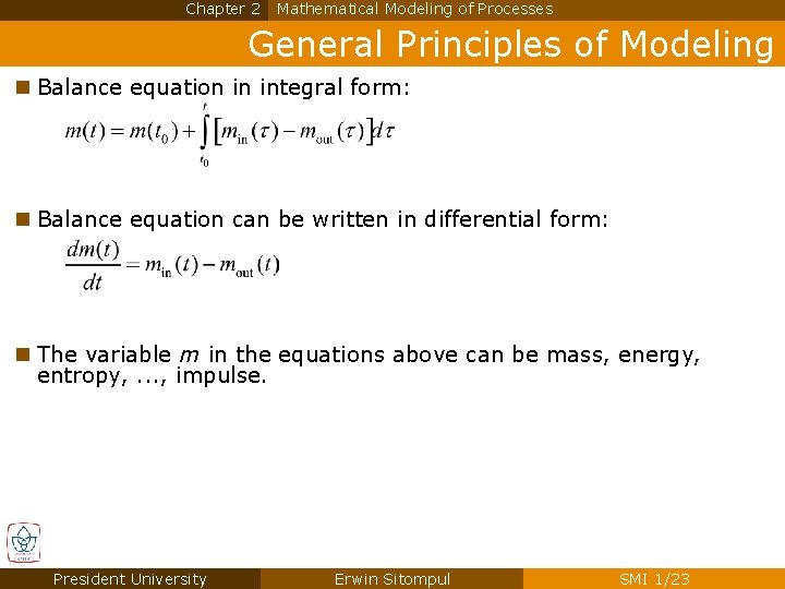
Chapter 2 Mathematical Modeling of Processes General Principles of Modeling n Balance equation in integral form: n Balance equation can be written in differential form: n The variable m in the equations above can be mass, energy, entropy, . . . , impulse. President University Erwin Sitompul SMI 1/23

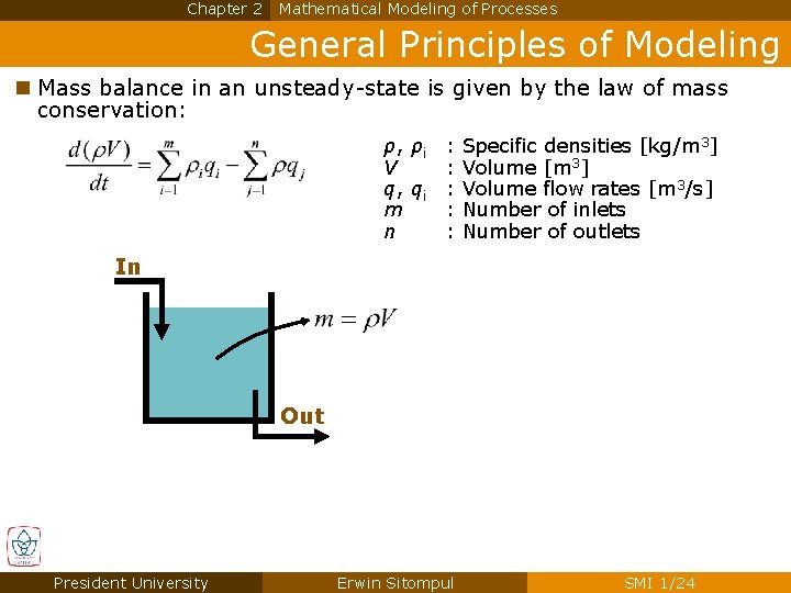
Chapter 2 Mathematical Modeling of Processes General Principles of Modeling n Mass balance in an unsteady-state is given by the law of mass conservation: ρ, ρi V q, qi m n : : : Specific densities [kg/m 3] Volume [m 3] Volume flow rates [m 3/s] Number of inlets Number of outlets In Out President University Erwin Sitompul SMI 1/24

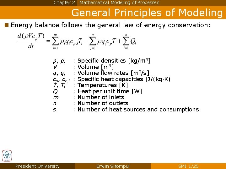
Chapter 2 Mathematical Modeling of Processes General Principles of Modeling n Energy balance follows the general law of energy conservation: ρ, ρi V q, qi cp, i T, Ti Q m n s President University : : : : : Specific densities [kg/m 3] Volume [m 3] Volume flow rates [m 3/s] Specific heat capacities [J/(kg K) Temperatures [K] Heat per unit time [W] Number of inlets Number of outlets Number of heat sources and consumptions Erwin Sitompul SMI 1/25

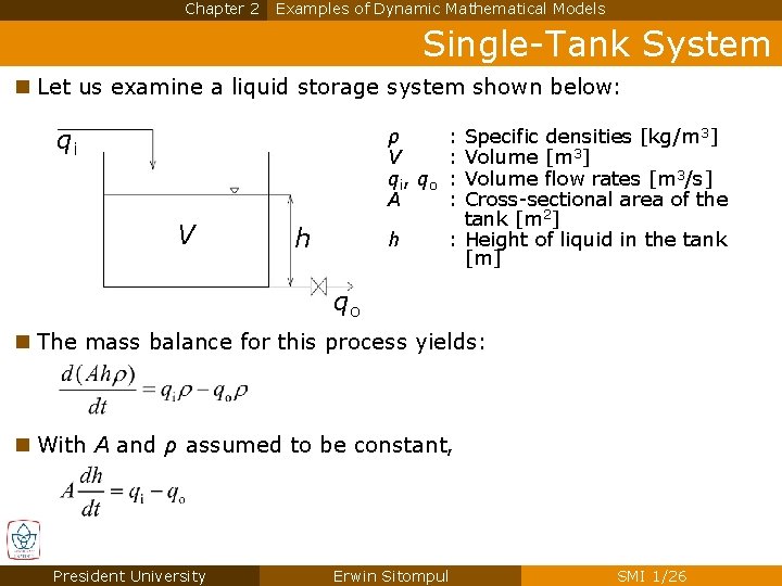
Chapter 2 Examples of Dynamic Mathematical Models Single-Tank System n Let us examine a liquid storage system shown below: qi ρ V qi, qo A V h h : : Specific densities [kg/m 3] Volume [m 3] Volume flow rates [m 3/s] Cross-sectional area of the tank [m 2] : Height of liquid in the tank [m] qo n The mass balance for this process yields: n With A and ρ assumed to be constant, President University Erwin Sitompul SMI 1/26

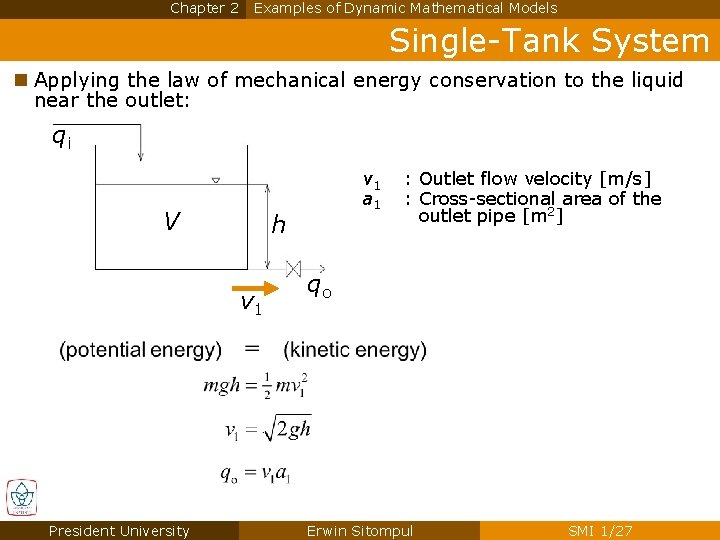
Chapter 2 Examples of Dynamic Mathematical Models Single-Tank System n Applying the law of mechanical energy conservation to the liquid near the outlet: qi V h v 1 President University v 1 a 1 : Outlet flow velocity [m/s] : Cross-sectional area of the outlet pipe [m 2] qo Erwin Sitompul SMI 1/27

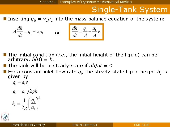
Chapter 2 Examples of Dynamic Mathematical Models Single-Tank System n Inserting q 0 = v 1 a 1 into the mass balance equation of the system: or n The initial condition (i. e. , the initial height of the liquid) can be arbitrary, h(0) = h 0. n The tank will be in steady-state if dh/dt = 0. n For a constant inlet flow rate qi, the steady-state liquid height hs is given by: President University Erwin Sitompul SMI 1/28

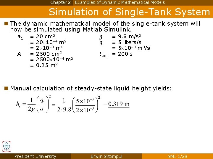
Chapter 2 Examples of Dynamic Mathematical Models Simulation of Single-Tank System n The dynamic mathematical model of the single-tank system will now be simulated using Matlab Simulink. a 1 A = = = 20 cm 2 20 10– 4 m 2 2 10– 3 m 2 2500 cm 2 2500 10– 4 m 2 0. 25 m 2 g qi tsim = = 9. 8 m/s 2 5 liters/s 5 10– 3 m 3/s 200 s n Manual calculation of steady-state liquid height yields: President University Erwin Sitompul SMI 1/29

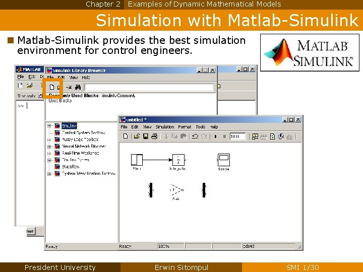
Chapter 2 Examples of Dynamic Mathematical Models Simulation with Matlab-Simulink n Matlab-Simulink provides the best simulation environment for control engineers. President University Erwin Sitompul SMI 1/30

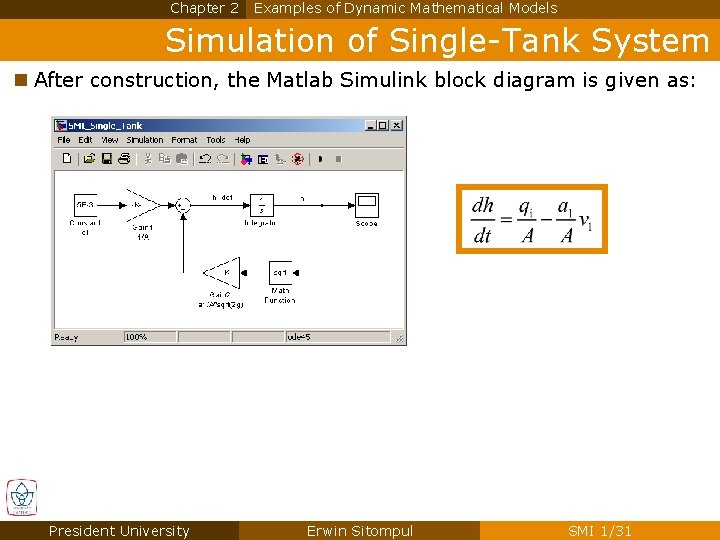
Chapter 2 Examples of Dynamic Mathematical Models Simulation of Single-Tank System n After construction, the Matlab Simulink block diagram is given as: President University Erwin Sitompul SMI 1/31

Chapter 2 Examples of Dynamic Mathematical Models Simulation of Single-Tank System n The simulation result, from transient until steady-state, can be observed by clicking the Scope. President University Erwin Sitompul SMI 1/32

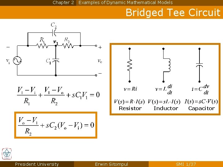
Chapter 2 Examples of Dynamic Mathematical Models Impulse and Charge Balance Equations n The impulse balance equation can be related to Newton’s law by: n The charge balance equation can be related to Kirchhoff's law by: President University Erwin Sitompul SMI 1/33

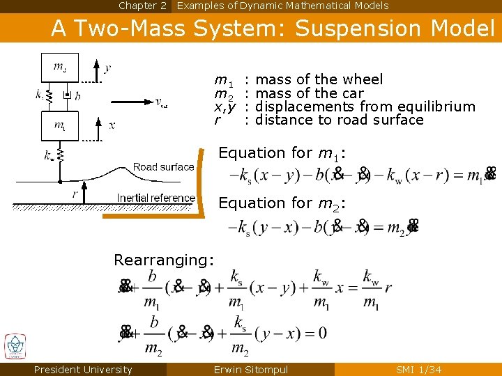
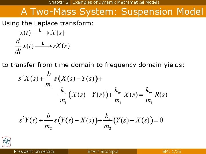
Chapter 2 Examples of Dynamic Mathematical Models A Two-Mass System: Suspension Model m 1 m 2 x, y r : : mass of the wheel mass of the car displacements from equilibrium distance to road surface Equation for m 1: Equation for m 2: Rearranging: President University Erwin Sitompul SMI 1/34

Chapter 2 Examples of Dynamic Mathematical Models A Two-Mass System: Suspension Model Using the Laplace transform: to transfer from time domain to frequency domain yields: President University Erwin Sitompul SMI 1/35

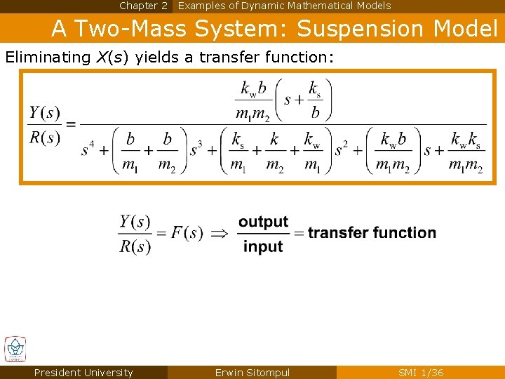
Chapter 2 Examples of Dynamic Mathematical Models A Two-Mass System: Suspension Model Eliminating X(s) yields a transfer function: President University Erwin Sitompul SMI 1/36

Chapter 2 Examples of Dynamic Mathematical Models Bridged Tee Circuit v 1 Resistor President University Erwin Sitompul Inductor Capacitor SMI 1/37

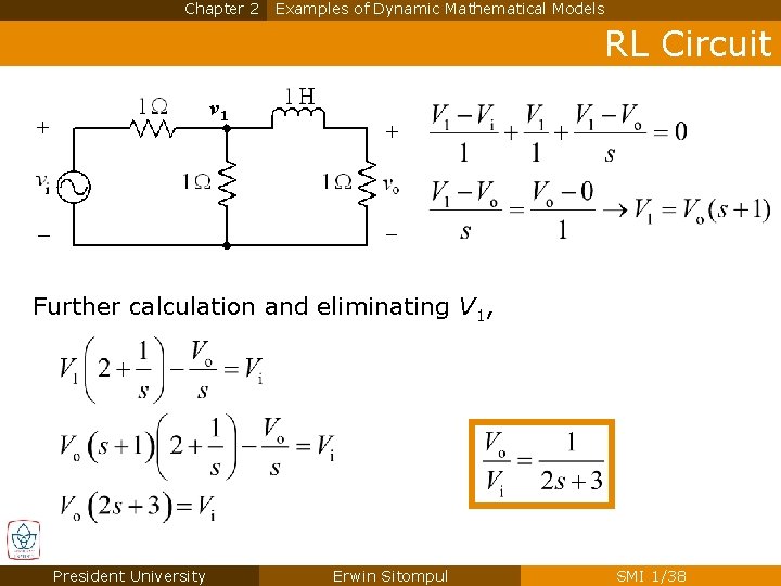
Chapter 2 Examples of Dynamic Mathematical Models RL Circuit v 1 Further calculation and eliminating V 1, President University Erwin Sitompul SMI 1/38

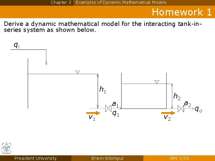
Chapter 2 Examples of Dynamic Mathematical Models Homework 1 Derive a dynamic mathematical model for the interacting tank-inseries system as shown below. qi h 1 v 1 President University a 1 q 1 Erwin Sitompul h 2 a 2 v 2 SMI 1/39 qo

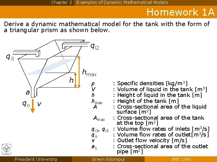
Chapter 2 Examples of Dynamic Mathematical Models Homework 1 A Derive a dynamic mathematical model for the tank with the form of a triangular prism as shown below. qi 2 qi 1 h a qo v President University hmax ρ V h hmax A : : : Amax : qi 1, qi 2 qo v a 1 : : Specific densities [kg/m 3] Volume of liquid in the tank [m 3] Height of liquid in the tank [m] Height of the tank [m] Cross-sectional area of the liquid surface [m 2] Cross-sectional area of the tank at the top [m 2] Volume flow rates of inlets [m 3/s] Volume flow rates of outlet[m 3/s] Outlet flow velocity [m/s] Cross-sectional area of the outlet pipe [m 2] Erwin Sitompul SMI 1/40