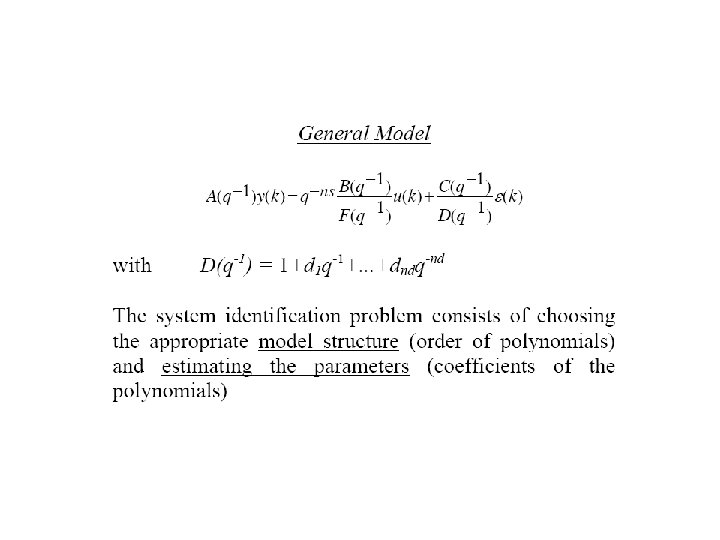
System identification and self regulating systems Discrete Equivalents


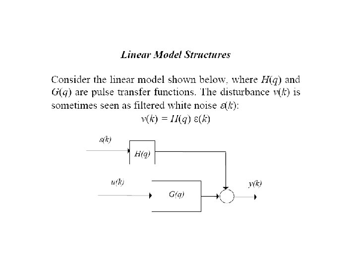
 e(t) + controller D(s) u(t) plant G(s) y(t) Translation")
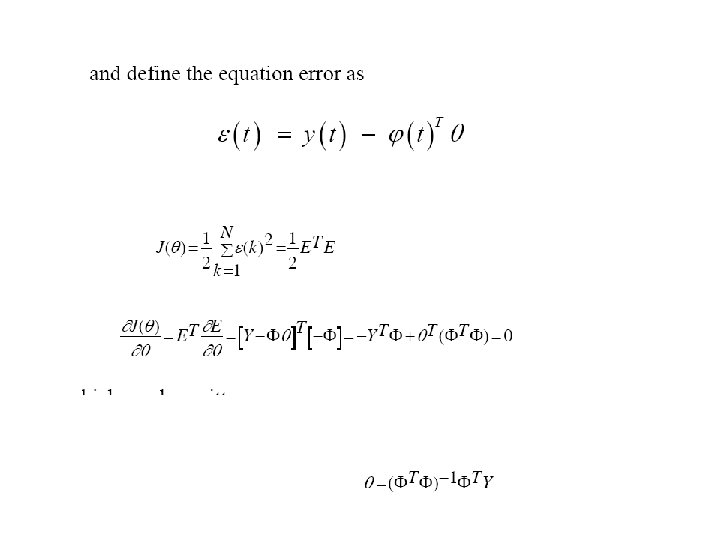
 as a differential equation. – Derive")


 • (Approximation k. T-T)")
")
 • (app ½(old value")
")


- Slides: 35
System identification and self regulating systems
Discrete Equivalents - Overview r(t) e(t) + controller D(s) u(t) plant G(s) y(t) Translation to discrete plant Translation to discrete controller (emulation) Zero order hold (ZOH) Numerical Integration • Forward rectangular rule • Backward rectangular rule • Trapeziod rule (Tustin’s method, bilinear transformation) • Bilinear with prewarping Emulation Zero-Pole Matching Purpose: Find a discrete transfer function which Hold Equivalents approximately has the same characteristics over • Zero order hold (ZOH) the frequency range of interest. • Triangle hold (FOH) Digital implementation: Control part constant between samples. Plant is not constant between samples.
Numerical Integration • Fundamental concept – Represent H(s) as a differential equation. – Derive an approximate difference equation. • We will use the following example – Notice, by partial expansion of a transfer function this example covers all real poles. Example Transfer function Differential equation
Numerical Integration
Numerical Integration • Now, three simple ways to approximate the area. k. T-T k. T – Forward rectangle • approx. by looking forward from k. T-T – Backward rectangle • approx. by looking backward from k. T – Trapezoid • approx. by average
Numerical Integration • Forward rectangular rule (Euler’s rule) • (Approximation k. T-T)
Numerical Integration • Backward rectangular rule (app k. T)
Numerical Integration • Trapezoid rule (Tustin’s Method, bilinear trans. ) • (app ½(old value + new value))
Numerical Integration • Comparison with H(s)
Numerical Integration • Transform s ↔ z • Comparison with respect to stability – In the s-plane, s = jw is the boundary between stability and instability.
The rest of this power point is not required in the exam Just for completeness purpose