System Components for the EASE Focus 3 Design

System Components for the EASE Focus 3 Design Project Amplifiers

Outline • Impedance matching in modern audio electronics • Amplifier power output vs. load impedance • How loudspeaker cable affects performance • Estimation of electrical power requirement • Clipping • Constant voltage speaker systems • Audio Power Amplifier Classes • A • B • AB • G • H • S/D • I

Impedance Matching in Audio Electronics • First, note that audio cables are not transmission lines, so “transmission line effects” (in general) do not apply • Examples: o A microphone output might be 150 , while a mic preamp input is typically 1 K or more o A guitar pickup output might be 100 K , while a guitar amp input is at least 1 M o A line level output will be something like 100 or less, while an (unbalanced) line level input is more like 10 K o A (good) solid state amplifier will have an output impedance less than 0. 5 , while the nominal impedance of a loudspeaker is at least 4 • For tube power amplifiers, however, the impedance of the output transformer secondary should be matched to the (nominal) loudspeaker (load) impedance in order to maximize power transfer

Amplifier Power Output vs. Load Impedance • Audio amplifier outputs are both voltage limited and current limited – they cannot output more power than the power supply can produce • Almost all audio amplifiers are voltage sources (output same voltage regardless of load impedance) – therefore, output power is a function of load impedance (which is a complex function that varies as a function of frequency): P = V x I x cos( ), where is the phase angle between the voltage and current delivered to the load • Power delivered to the load will therefore double if the load impedance is halved…as long as the power supply does not run out of current

Amplifier Power Output vs. Load Impedance • Example: • Class D amplifier with 15 VDC, 4 A power supply • The maximum peak-to-peak output voltage that can be produced is 15 VDC (minus the voltage drop across each of the power MOSFETs) • For reproducing a sine wave, the maximum RMS output voltage is 10. 61 VAC • The amplifier will produce this same output voltage swing regardless of load impedance until it runs out of current • P = V 2 / R 28 W RMS @ 4 (I = 2. 64 A) , 14 W RMS @ 8 (I = 1. 32 A) • What happens if load impedance is reduced to 2 ? Ø In theory, P = 56 W RMS, but that would require the power supply to produce 5. 28 A of current @ 15 VDC, which is beyond its rated capability Ø The absolute maximum power that can be delivered to the load is therefore 42. 4 W RMS, with a load impedance of 2. 66 (assuming 100% efficiency) Ø If the amplifier is 90% efficient (typical of Class D), the maximum power that can be delivered is about 38 W RMS, at a minimum load impedance of 3

Amplifier Power Output vs. Load Impedance

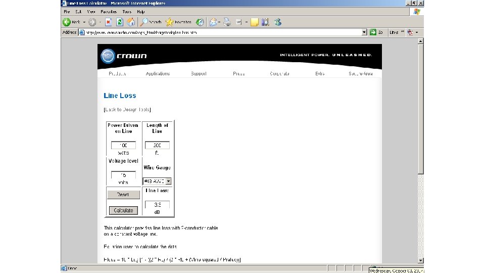
How Loudspeaker Cable Affects Performance • Damping is a measure of a power amplifier's ability to control the back EMF motion of the loudspeaker cone after the signal disappears • The damping factor of a system is the ratio of the loudspeaker's nominal impedance to the total impedance driving it • Example: Amplifier with damping factor of 300 (bigger is better) driving an 8 load means that the output impedance is 0. 027 (lower is better) • Impedance of speaker cable used can significantly reduce the damping factor (larger gauge wire has lower impedance)

Estimation of Electrical Power Requirement • When SPL goal at a given listening distance known, also need: • Sensitivity rating of loudspeaker (typically spec as 1 m on-axis with input of 1 electrical watt) • Acoustic level change/attenuation between loudspeaker and farthest listening position • Example: 90 d. B program level at listening distance of 32 m outdoors • Loudspeaker sensitivity measured as 110 d. B • Acoustic level change = 20 log (32) 30 d. B • Add 10 d. B for peak (program level) headroom • SPL required at source is 90 + 30 + 10 = 130 d. B • Need 20 d. B above 1 watt, or 10 (20/10) = 100 W

http: //www. crownaudio. com

Clipping • Clipping is distortion caused when one or more audio output waveforms are driven beyond the voltage swing provided by the amplifier’s power supply • Short-term (transient) clipping is a result of insufficient peak power available • Long-term clipping is a result of inadequate continuous (RMS) power available for the desired level setting • “Hard” clipping produces high-order harmonics that can damage loudspeakers • Note that clipping can be asymmetric due to bias level of output devices

Constant Voltage Speaker Systems • Constant voltage (aka “ 70 volt” or “high voltage”) speaker systems consist of loudspeakers connected in parallel via “step-down” transformers • Each step-down transformer has multiple power taps to control the relative volume level at each speaker (variable attenuators are available as well) • Utilize higher voltage/lower current to distribute signal using smaller gauge wire (voltage is “stepped up” at the amplifier – transformer may not be required) • Unique capabilities: Typical line values for a 100 watt amplifier are 70 V, 1. 41 A, and 50 o Drive many loudspeakers from a single power amplifier o Wired in parallel (can be “daisy-chained”) o Use relatively small gauge cable o Can set relatively level of each loudspeaker independently o Ideal for distributed/delayed “fill” systems and ceiling speakers

Audio Power Amplifier Classes • Audio power amplifiers were originally classified according to the relationship between the output voltage swing and the input voltage swing • Classification was based on the amount of time the output devices operate during one complete cycle of a signal swing • Classes were also defined in terms of output bias current (the amount of current flowing in the output devices with no applied signal) • For discussion purposes (with the exception of class A), assume a simple output stage consisting of two complementary devices (one positive polarity and one negative polarity) using any type of transistor (e. g. BJT or MOSFET)

Power Amplifier Classes – “A” • Class “A” • key ingredient of class A operation is that output device is always on • single-ended design with only one type polarity output device • the most inefficient of all power amplifier designs, averaging only around 20% (large, heavy, and run very hot) • are inherently the most linear, with the least amount of distortion • impractical for professional audio applications due to inefficiency

Class A: Vacuum Tube Single-Ended • Single power vacuum tube • A transformer is used to isolate the high voltage DC V+ from the load and match the loudspeaker load impedance various possible load lines Reference: https: //www. vtadiy. com/book/chapter-4 -integrated-push-pull-vacuumtube-amplifier/4 -1 -output-stage-or-power-stage/4 -1 -1 -single-ended-configuration/

Class A: Transistor Single-Ended • Common emitter circuit large voltage gain • A transformer can be used to improve efficiency • A large coupling capacitor may be necessary to remove DC bias from the loudspeaker output Reference: https: //www. electronics-tutorials. ws/amplifier/amp_5. htmln/

Example: Class A Accuphase A-47 $17, 500 = 45 watts/channel into 8

Power Amplifier Classes – “B” • Class “B” • opposite of class A: both output devices are never allowed to be on at the same time • each output device is on for exactly one half of a complete sinusoidal signal cycle • class B designs show high efficiency but poor linearity around the crossover region (due to the time it takes to turn one device off and the other device on, which translates into extreme crossover distortion ) • class B designs restricted to low power applications, e. g. , battery operated equipment, such as communications audio

Class A vs. Class B Vcc crossover distortion output transistors are not “pre-biased” to an “ON” state of operation – each transistor only conducts when the input signal exceeds VBE

Power Amplifier Classes – “AB” • Class “AB” • intermediate case: both devices are allowed to be on at the same time, but just barely • output bias is set so that current flows in a specific output device appreciably more than a half cycle but less than the entire cycle (enough to keep each device operating so they respond instantly to input voltage demands) • the inherent non-linearity of class B designs is eliminated, without the gross inefficiencies of the class A design • combination of good efficiency (around 50%) with excellent linearity that makes class AB the most popular consumer audio amplifier design

Basic Class AB Power Amplifier Output Stage output transistors are “pre-biased” to a “barely ON” state of operation – greatly reduces crossover distortion dual-rail (+/-) power supply single rail power supply, adj. bias vs. diode biasingle rail power supply, driver stage with diode biasing

Vacuum Tube Push-Pull (Class AB) • Two power vacuum tubes (e. g. 6 L 6 GC, EL 34/6 CA 7) are used to amplify phase-inverted copies of the same signal • The amplified signals are combined together using a centertapped transformer, which is used to match the load impedance • Cancels power supply noise and clips symmetrically (“musically”) Reference: https: //www. vtadiy. com/book/chapter-4 -integrated-push-pull-vacuumtube-amplifier/4 -1 -output-stage-or-power-stage/4 -1 -4 -push-pull-configuration/ quiescent operating point

Example: Class AB

Power Amplifier Classes – “G” • Class “G” • operation involves changing the power supply voltage from a lower level to a higher level when larger output swings are required • common for pro audio designs • several ways to do this: • simplest involves a single class AB output stage that is connected to two power supply rails by a diode or transistor • for most musical program material, the output stage is connected to the lower supply voltage • automatically switches to the higher rails for large signal peaks (thus the nickname rail-switcher) • Another approach uses two class AB output stages, each connected to a different power supply voltage • the magnitude of the input signal determines the signal path • use of two power supplies improves efficiency enough to allow significantly more power for a given size/weight

Class G Amplifier Rail Switching

Power Amplifier Classes – “H” • Class “H” • takes the class G design one step further and actually modulates the higher power supply voltage by the input signal • allows the power supply to track the audio input and provide just enough voltage for optimum operation of the output devices (thus the nickname rail-tracker or tracking power amplifier) • the efficiency of class H is comparable to class G designs

Class H Tracking Power Supply

Example: Class H

Comparison of Linear Amplifier Relative Efficiency wasted power AB G 2 G 3 H

Power Amplifier Classes – “S” • Class “S” • first invented in 1932 • used for both amplification and amplitude modulation • similar to Class D except the rectangular PWM voltage waveform is applied to a low-pass filter that allows only the slowly varying DC or average voltage component to appear across the load • essentially this is what is called “Class D” today

Power Amplifier Classes – “D” • Class “D” • operation is switching, hence the term switching power amplifier • output devices are rapidly switched on and off at least twice for each cycle • the output devices are either completely on or completely off so theoretically they do not dissipate any power • class D operation is theoretically 100% efficient, but this requires zero on-impedance (MOSFET) switches with infinitely fast switching times • practical designs do exist with true efficiencies approaching 90% • Class D is at least as old as 1954 (U. S. Patent 2, 821, 639: solidstate full-bridge servo amplifier)

Basic Class D Principle

Power Amplifier Classes – “D” • Class “D” – Complications • need to operate at high switching speed (e. g. , 250 KHz) for full audio bandwidth (20 KHz) reproduction with low distortion • traditional design requires “dead time” between positive and negative polarity phases (to avoid destruction of output switching devices) – introduces additional distortion • quality of switching devices (“on” resistance, switching speed) limit efficiency/performance

Example: Class D

Example: Class D

Relative Efficiency of Class D vs. Linear Amplifiers Class D Class H Class G 3 Class G 2 Class AB

Power Amplifier Classes – “I” • Class “I” • based on patent U. S. 5, 657, 219 covering opposed current converters • "I" is short for "interleave" as this is the only four-quadrant converter known that uses two switches yet that has an interleave number of 2 • when used with fixed-frequency naturally sampled twosided PWM it forms a theoretically optimum converter having the least unnecessary/undesirable PWM spectra • also called a “balanced current amplifier”

Balanced Current Switching Amplifier

Example: Class I

Industry Trends • Analog amplifier (“Class AB”) market share $2 -3 B in 2003 (Class D market share was only 2 -3%) • By 2006, digital amplifier (“Class D”) market share rose to 15%, by 2008 to 30%, by 2011 67% • Global class D amplifier market is expected to grow 14% during 2016 -2022