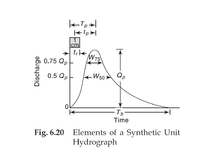
Synthetic UH Definition Synthetic Hydrograph is a plot

Synthetic UH • Definition: Synthetic Hydrograph is a plot of flow versus time and generated based on a minimal use of streamflow data. • Example: A pending land use change and the resulting runoff hydrograph is thus unknown, but nevertheless must be estimated.

Synthetic UH • Developed for basin that were ungauged • Based on data from similar gauged basins • Most methods are very similar in nature • Revolutionized ability to predict hydro response

Gauged and ungauged watersheds • Gauged watersheds – Watersheds where data on precipitation, streamflow, and other variables are available • Ungauged watersheds – Watersheds with no data on precipitation, streamflow and other variables.

Need for synthetic UH • UH is applicable only for gauged watershed and for the point on the stream where data are measured • For other locations on the stream in the same watershed or for nearby (ungauged) watersheds, synthetic procedures are used.

Synthetic UH • Synthetic hydrographs are derived by – Relating hydrograph characteristics such as peak flow, base time etc. with watershed characteristics such as area and time of concentration. – Using dimensionless unit hydrograph – Based on watershed storage

Synthetic UH Methods • Snyder’s Method (1938) • Clark Method (1945) • Nash (1958) • SCS (1964, 1975) • Espey-Winslow (1968) • Kinematic Wave (1970 s)

Snyder’s Method • Synder (1938)- based on study of large catchment in eastern US developed a set of empirical equation for synthetic UH. • The equation are use in USA and with some modification in many other countries.

Snyder’s Methods to characterize ungaged basins - 1938 Use data and relationships developed from gages Variety of approaches but most based on tp and Qp, Where tp = lag time (hr) and Qp = peak flow in cms/cfs

Snyder’s Equation tp = Ct (LLca)0. 3 • tp=basin lag in hour • L= basin length in km • Lca= distance along the main water course from gauging stn. To a point opposite to the watershed centroid in km • Ct = regional constant represent watershed slope and storage effects.

Lag time • The most important characteristic of basin due to storm- basin lag (lag time) • Lag time- time difference between the centroid of the input (rainfall excess) and the output (DRH) • Represent time of travel of water from all parts of watershed to the outlet during a given storm.

Snyder’s UH Method

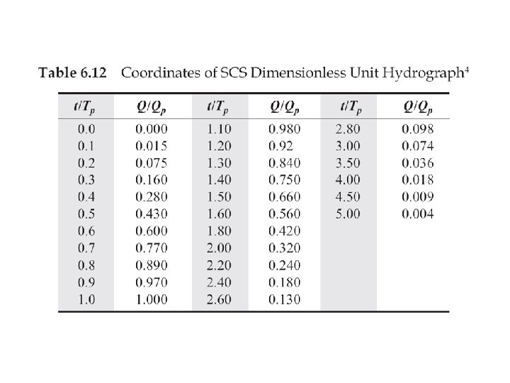
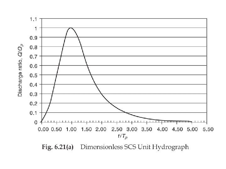
SCS Method • Dimensionless UH • Based on a study of large number of UH • Developed by US Soil Conservation Services (SCS)

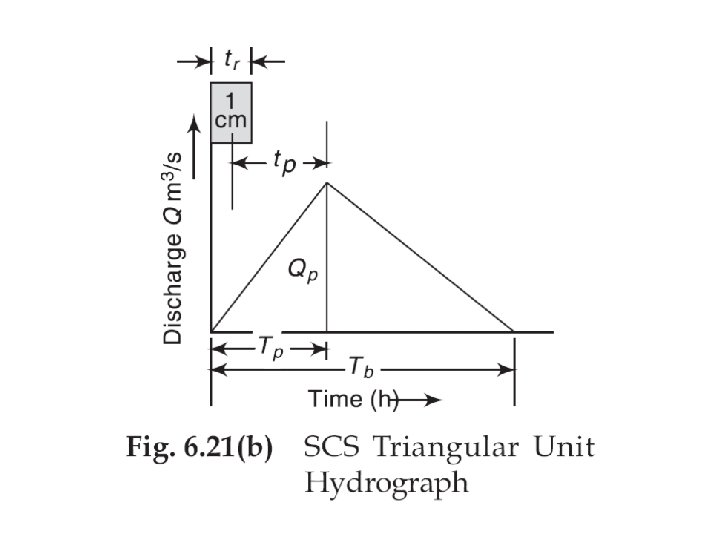
The SCS Unit Hydrograph 1. For large watersheds, time of concentration tc duration (D) of constant rainfall intensity 2. Rainfall cannot last long enough that the peak flow, Qp, will occur at time tc 3. Instead, the peak flow, Qp, will occur at time tp, which is a function of rainfall duration D and the watershed characteristics represented by tc

Triangular UH SCS Methods Dimensionless UH

SCS dimensionless hydrograph • Synthetic UH in which the discharge is expressed by the ratio of q to qp and time by the ratio of t to Tp • If peak discharge and lag time are known, UH can be estimated. Tc: time of concentration C = 2. 08 (483. 4 in English system) A: drainage area in km 2 (mi 2)

Ex. 7. 7. 3 • Construct a 10 -min SCS UH. A = 3. 0 km 2 and Tc = 1. 25 h 0. 833 h q Multiply y-axis of SCS hydrograph by qp and x-axis by Tp to get the required UH, or construct a triangular UH 7. 49 m 3/s. cm 2. 22 h t

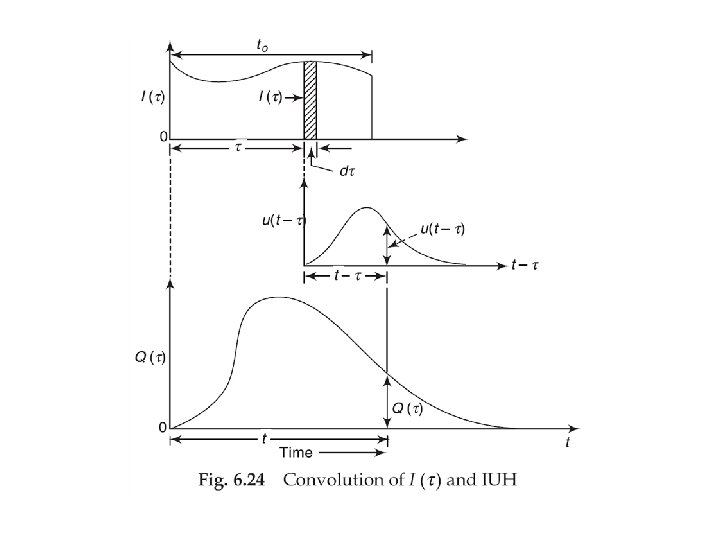
Clark Unit Hydrograph (UH) Computation • Based on the use of time-area method. • Concept of instantaneous unit hydrograph (IUH)

Clark Unit Hydrograph (UH) Computation • Figure 6. 23 shows the shape of different hydrographs for different D values. • As D is reduced, the intensity of rainfall excess being equal to 1/D increases and the UH becomes more skewed. • A finite UH indicated as D 0. • The limiting case of UH of zero duration is known as instantaneous unit hydrograph (IUH).

Method of IUH 1. Develop a time area (TA) curve 2. Route the time area curve through a linear reservoir with a Clark routing parameter

Example 6. 16

Nash Linear model

Kinematic Wave Overland Collector Channels Main Stream Manning’s Eqn

Kinematic Wave