Symmetric Difference Quotient The Symmetric Difference Quotient 2

- Slides: 9

Symmetric Difference Quotient

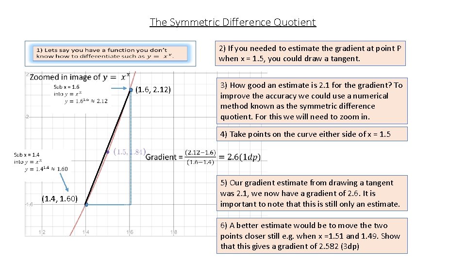
The Symmetric Difference Quotient 2) If you needed to estimate the gradient at point P when x = 1. 5, you could draw a tangent. (1. 6, 2. 12) (3, 5) (1. 5, 1. 84) P (1. 4, 1. 60) 3) How good an estimate is 2. 1 for the gradient? To improve the accuracy we could use a numerical method known as the symmetric difference quotient. For this we will need to zoom in. 4) Take points on the curve either side of x = 1. 5 5) Our gradient estimate from drawing a tangent was 2. 1, we now have a gradient of 2. 6. It is important to note that this is still only an estimate. 6) A better estimate would be to move the two points closer still e. g. when x =1. 51 and 1. 49. Show that this gives a gradient of 2. 582 (3 dp)

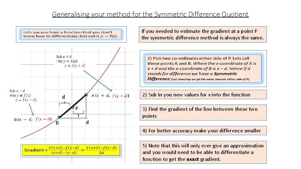
Generalising your method for the Symmetric Difference Quotient If you needed to estimate the gradient at a point P the symmetric difference method is always the same. A d d PP B B dd 2) Sub in you new values for x into the function 3) Find the gradient of the line between these two points 4) For better accuracy make your difference smaller 5) Note that this will only ever give an approximation and you would need to be able to differentiate a function to get the exact gradient.

Now You try Print of slides 5 -9, for each function you can draw a tangent to estimate a gradient and then improve your answer with the symmetric difference quotient. Remember that reducing the size of the difference will improve the accuracy of the gradient. If the function is something that you know how to differentiate then you can use your “algebraic technique” to do this. This will give you an exact answer. It is important to understand the phrases “numerical technique” and “algebraic technique” as exam questions may refer to them in this way.

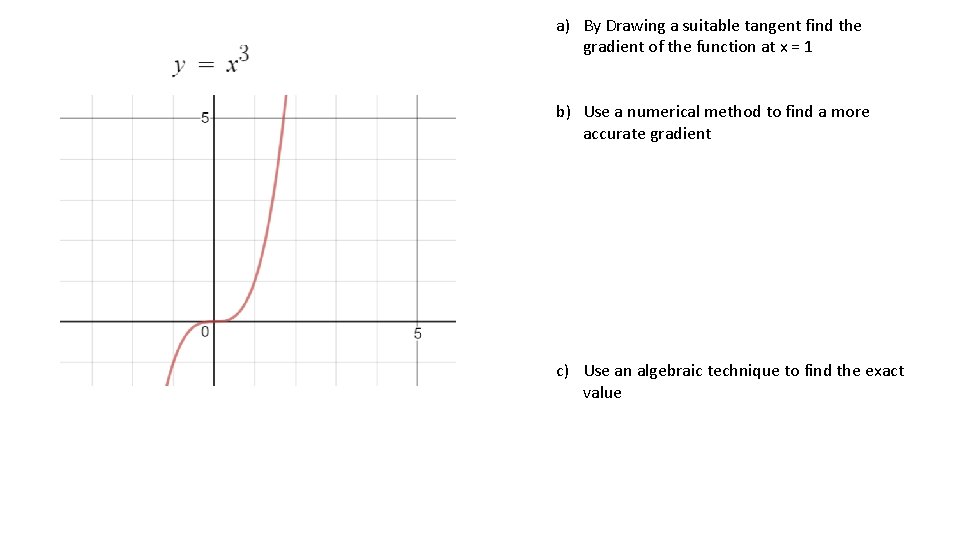
a) By Drawing a suitable tangent find the gradient of the function at x = 1 b) Use a numerical method to find a more accurate gradient c) Use an algebraic technique to find the exact value

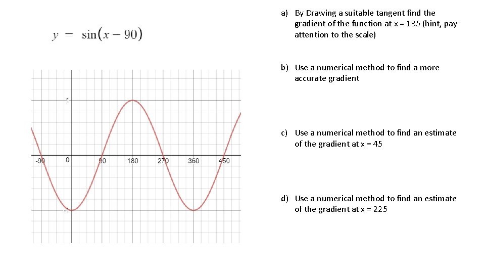
a) By Drawing a suitable tangent find the gradient of the function at x = 135 (hint, pay attention to the scale) b) Use a numerical method to find a more accurate gradient c) Use a numerical method to find an estimate of the gradient at x = 45 d) Use a numerical method to find an estimate of the gradient at x = 225

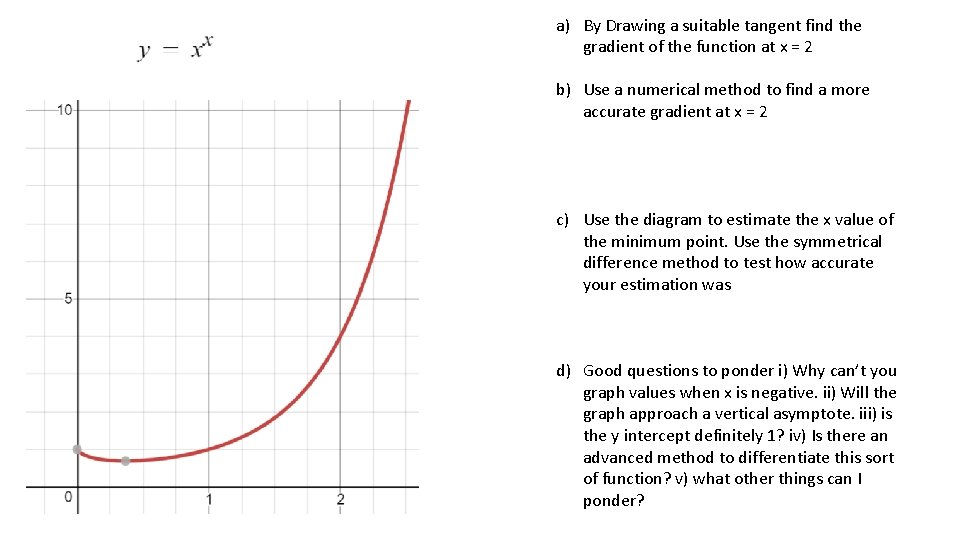
a) By Drawing a suitable tangent find the gradient of the function at x = 2 b) Use a numerical method to find a more accurate gradient at x = 2 c) Use the diagram to estimate the x value of the minimum point. Use the symmetrical difference method to test how accurate your estimation was d) Good questions to ponder i) Why can’t you graph values when x is negative. ii) Will the graph approach a vertical asymptote. iii) is the y intercept definitely 1? iv) Is there an advanced method to differentiate this sort of function? v) what other things can I ponder?

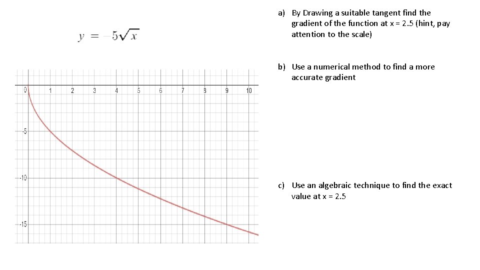
a) By Drawing a suitable tangent find the gradient of the function at x = 2. 5 (hint, pay attention to the scale) b) Use a numerical method to find a more accurate gradient c) Use an algebraic technique to find the exact value at x = 2. 5

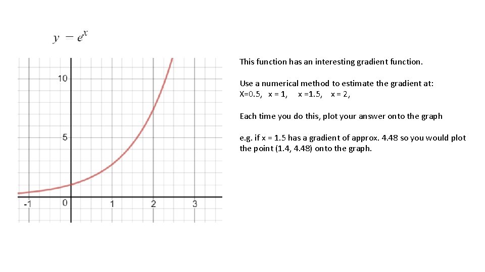
This function has an interesting gradient function. Use a numerical method to estimate the gradient at: X=0. 5, x = 1, x =1. 5, x = 2, Each time you do this, plot your answer onto the graph e. g. if x = 1. 5 has a gradient of approx. 4. 48 so you would plot the point (1. 4, 4. 48) onto the graph.