Switching Forwarding and Routing Network layer functions r

Switching, Forwarding and Routing

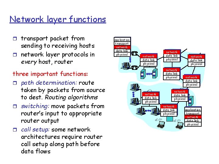
Network layer functions r transport packet from sending to receiving hosts r network layer protocols in every host, router three important functions: r path determination: route taken by packets from source to dest. Routing algorithms r switching: move packets from router’s input to appropriate router output r call setup: some network architectures require router call setup along path before data flows application transport network data link physical network data link physical network data link physical application transport network data link physical

Network service model service abstraction Q: What service model for “channel” transporting packets from sender to receiver? r guaranteed bandwidth? r preservation of inter-packet timing (no jitter)? r loss-free delivery? r in-order delivery? r congestion feedback to sender? The most important abstraction provided by network layer: ? ? ? virtual circuit or datagram?

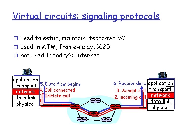
Virtual circuits “source-to-dest path behaves much like telephone circuit” m m performance-wise network actions along source-to-dest path r call setup, teardown for each call before data can flow r each packet carries VC identifier (not destination host OD) r every router on source-dest path s maintain “state” for each passing connection m transport-layer connection only involved two end systems r link, router resources (bandwidth, buffers) may be allocated to VC m to get circuit-like perf.

Virtual circuits: signaling protocols r used to setup, maintain teardown VC r used in ATM, frame-relay, X. 25 r not used in today’s Internet application transport 5. Data flow begins network 4. Call connected data link 1. Initiate call physical 6. Receive data application 3. Accept call transport 2. incoming call network data link physical

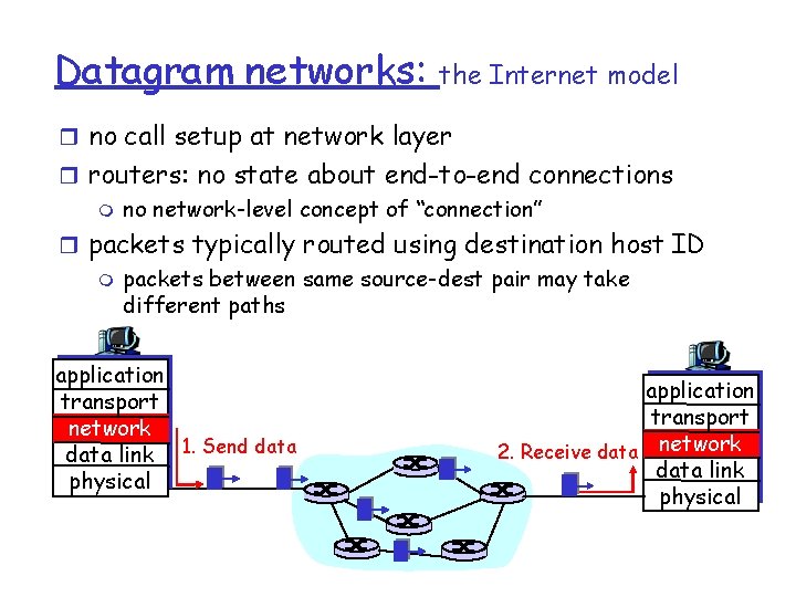
Datagram networks: the Internet model r no call setup at network layer r routers: no state about end-to-end connections m no network-level concept of “connection” r packets typically routed using destination host ID m packets between same source-dest pair may take different paths application transport network data link 1. Send data physical application transport 2. Receive data network data link physical

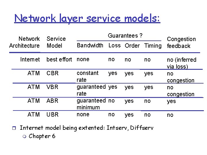
Network layer service models: Network Architecture Internet Service Model Guarantees ? Congestion Bandwidth Loss Order Timing feedback best effort none ATM CBR ATM VBR ATM ABR ATM UBR constant rate guaranteed minimum none no no no yes yes yes no no (inferred via loss) no congestion yes no no r Internet model being extented: Intserv, Diffserv m Chapter 6

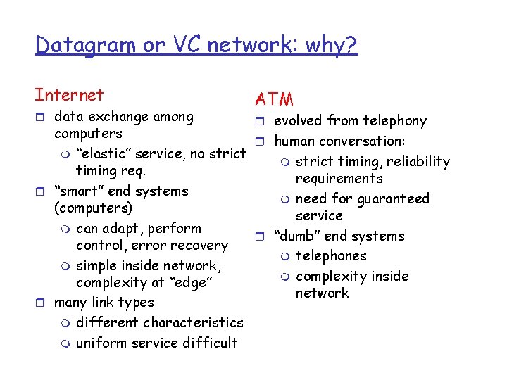
Datagram or VC network: why? Internet r data exchange among ATM r evolved from telephony computers r human conversation: m “elastic” service, no strict m strict timing, reliability timing requirements r “smart” end systems m need for guaranteed (computers) service m can adapt, perform r “dumb” end systems control, error recovery m telephones m simple inside network, m complexity inside complexity at “edge” network r many link types m different characteristics m uniform service difficult

Routing r The primary function of a packet network is to accept packets from a source and deliver them to a destination node. r The process of forwarding the packets through the network is referred to a routing. r Routing mechanisms have a set of requirements: m m m correctness simplicity robustness stability fairness

r Most important: m optimality m efficiency r Routing directly impacts the performance of the network! WHY? r In order to route packets on optimal routes through the network to their destinations, we must first decide what is to be optimized: m m m delay cost throughput

r Routing decisions are generally based on some knowledge of the state of the network. m Delay on certain links m Cost through certain nodes m Packet loss m etc. r This information may have to be dynamically collected. This leads to overhead which in turn reduces the utilization.

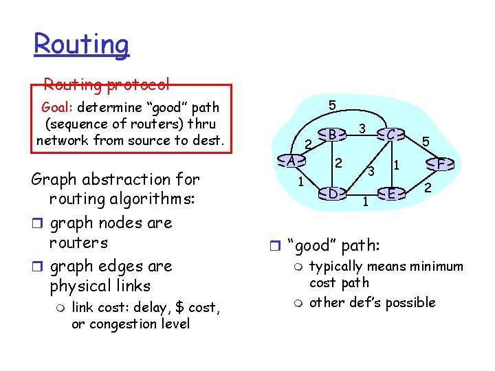
Routing protocol 5 Goal: determine “good” path (sequence of routers) thru network from source to dest. Graph abstraction for routing algorithms: r graph nodes are routers r graph edges are physical links m link cost: delay, $ cost, or congestion level 2 A B 2 1 D 3 C 3 1 5 F 1 E 2 r “good” path: m typically means minimum cost path m other def’s possible

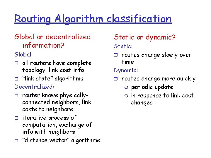
Routing Algorithm classification Global or decentralized information? Global: r all routers have complete topology, link cost info r “link state” algorithms Decentralized: r router knows physicallyconnected neighbors, link costs to neighbors r iterative process of computation, exchange of info with neighbors r “distance vector” algorithms Static or dynamic? Static: r routes change slowly over time Dynamic: r routes change more quickly m periodic update m in response to link cost changes

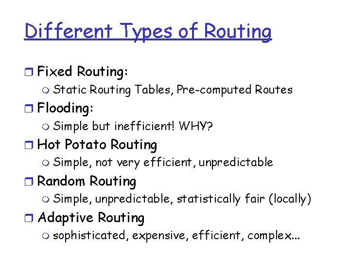
Different Types of Routing r Fixed Routing: m Static Routing Tables, Pre-computed Routes r Flooding: m Simple but inefficient! WHY? r Hot Potato Routing m Simple, not very efficient, unpredictable r Random Routing m Simple, unpredictable, statistically fair (locally) r Adaptive Routing m sophisticated, expensive, efficient, complex. . .

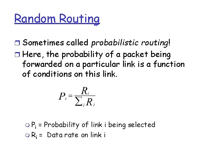
Random Routing r Sometimes called probabilistic routing! r Here, the probability of a packet being forwarded on a particular link is a function of conditions on this link. m Pi = Probability of link i being selected m Ri = Data rate on link i

r Note: Random Routing is probabilistic, i. e. , the link with the largest capacity may not be the one chosen for every transmission. r We can formulate a static and dynamic (adaptive) version of the routing algorithm. r Can you think of other measurements (metrics) to compute Pi ?

Adaptive Routing r Adaptive Routing Techniques are used in almost all packet-switching networks. m ARPANET r Routing decisions change in response to changes in the network. m m Network Failure Congestion r Adaptive routing strategies can improve performance. r Adaptive routing strategies can aid congestion control.

r Adaptive routing mechanisms are based on shortest path algorithm usually developed in the field of graph theory. r The trick is to formulate the centralized form of these algorithm to work in a distributed setting, such as a communication network. r The information upon routing decisions are based may come from m local measurements adjacent nodes all nodes in the network

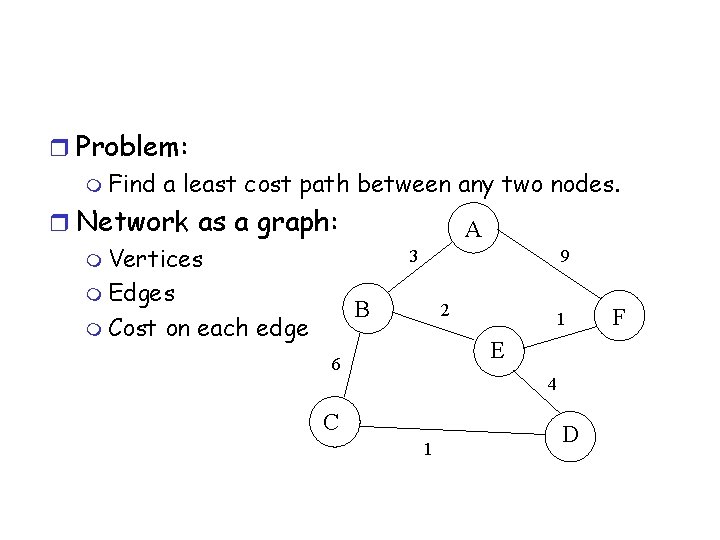
r Problem: m Find a least cost path between any two nodes. r Network as a graph: m Vertices m Edges B m Cost on each edge A 3 9 2 1 E 6 4 C 1 D F

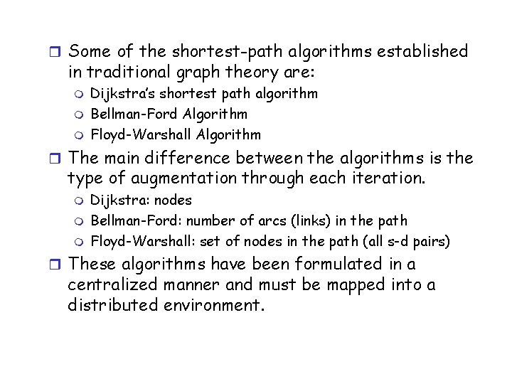
r Some of the shortest-path algorithms established in traditional graph theory are: m m m Dijkstra’s shortest path algorithm Bellman-Ford Algorithm Floyd-Warshall Algorithm r The main difference between the algorithms is the type of augmentation through each iteration. m m m Dijkstra: nodes Bellman-Ford: number of arcs (links) in the path Floyd-Warshall: set of nodes in the path (all s-d pairs) r These algorithms have been formulated in a centralized manner and must be mapped into a distributed environment.

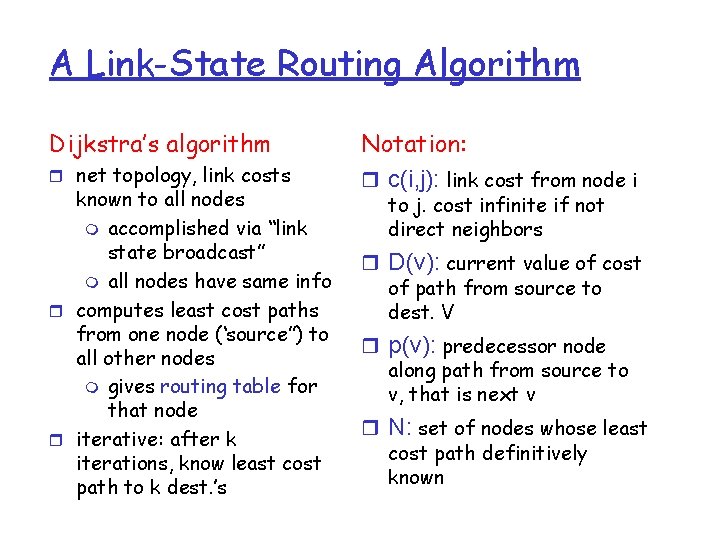
A Link-State Routing Algorithm Dijkstra’s algorithm r net topology, link costs known to all nodes m accomplished via “link state broadcast” m all nodes have same info r computes least cost paths from one node (‘source”) to all other nodes m gives routing table for that node r iterative: after k iterations, know least cost path to k dest. ’s Notation: r c(i, j): link cost from node i to j. cost infinite if not direct neighbors r D(v): current value of cost of path from source to dest. V r p(v): predecessor node along path from source to v, that is next v r N: set of nodes whose least cost path definitively known

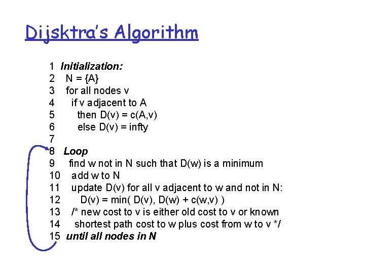
Dijsktra’s Algorithm 1 Initialization: 2 N = {A} 3 for all nodes v 4 if v adjacent to A 5 then D(v) = c(A, v) 6 else D(v) = infty 7 8 Loop 9 find w not in N such that D(w) is a minimum 10 add w to N 11 update D(v) for all v adjacent to w and not in N: 12 D(v) = min( D(v), D(w) + c(w, v) ) 13 /* new cost to v is either old cost to v or known 14 shortest path cost to w plus cost from w to v */ 15 until all nodes in N

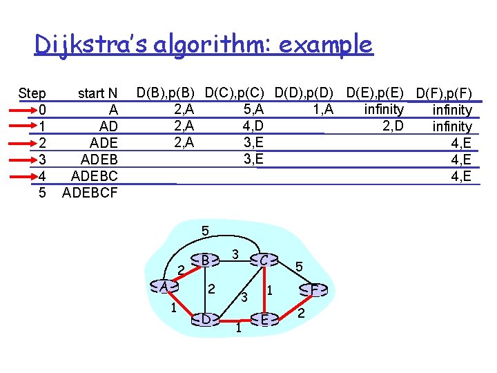
Dijkstra’s algorithm: example Step 0 1 2 3 4 5 start N A AD ADEBCF D(B), p(B) D(C), p(C) D(D), p(D) D(E), p(E) D(F), p(F) 2, A 1, A 5, A infinity 2, A 4, D 2, D infinity 2, A 3, E 4, E 5 2 A B 2 1 D 3 C 3 1 5 F 1 E 2

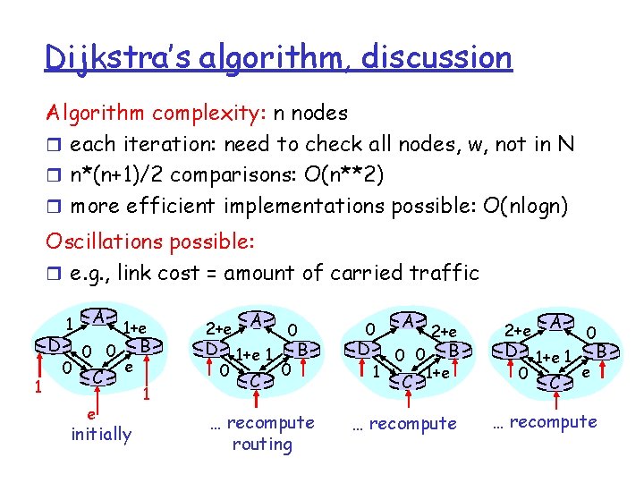
Dijkstra’s algorithm, discussion Algorithm complexity: n nodes r each iteration: need to check all nodes, w, not in N r n*(n+1)/2 comparisons: O(n**2) r more efficient implementations possible: O(nlogn) Oscillations possible: r e. g. , link cost = amount of carried traffic D 1 1 0 A 0 0 C e 1+e e initially B 1 2+e A 0 D 1+e 1 B 0 0 C … recompute routing 0 D 1 A 0 0 C 2+e B 1+e … recompute 2+e A 0 D 1+e 1 B e 0 C … recompute

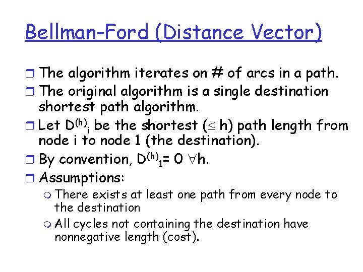
Bellman-Ford (Distance Vector) r The algorithm iterates on # of arcs in a path. r The original algorithm is a single destination shortest path algorithm. r Let D(h)i be the shortest ( h) path length from node i to node 1 (the destination). r By convention, D(h)1= 0 h. r Assumptions: m There exists at least one path from every node to the destination m All cycles not containing the destination have nonnegative length (cost).

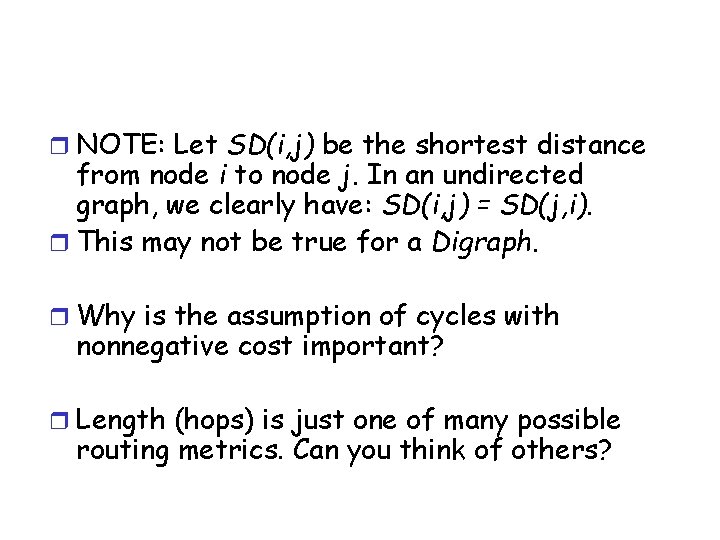
r NOTE: Let SD(i, j) be the shortest distance from node i to node j. In an undirected graph, we clearly have: SD(i, j) = SD(j, i). r This may not be true for a Digraph. r Why is the assumption of cycles with nonnegative cost important? r Length (hops) is just one of many possible routing metrics. Can you think of others?

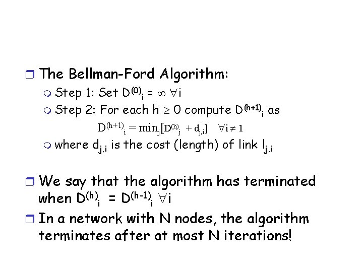
r The Bellman-Ford Algorithm: m Step 1: Set D(0)i = i m Step 2: For each h 0 compute D(h+1)i as D(h+1)i = minj[D(h)j + dj, i] i 1 m where dj, i is the cost (length) of link lj, i r We say that the algorithm has terminated when D(h)i = D(h-1)i i r In a network with N nodes, the algorithm terminates after at most N iterations!

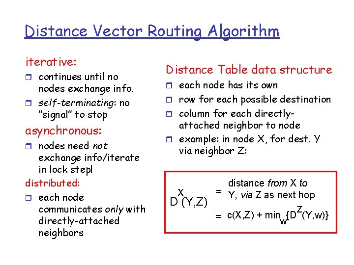
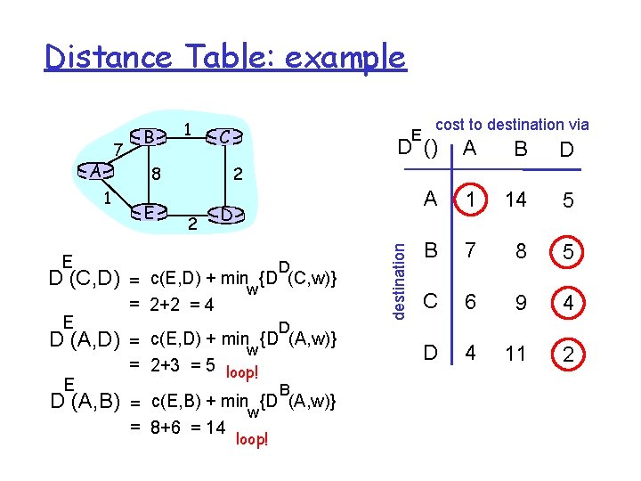
Distance Vector Routing Algorithm iterative: r continues until no nodes exchange info. r self-terminating: no “signal” to stop asynchronous: r nodes need not exchange info/iterate in lock step! distributed: r each node communicates only with directly-attached neighbors Distance Table data structure r each node has its own r row for each possible destination r column for each directly- attached neighbor to node r example: in node X, for dest. Y via neighbor Z: X D (Y, Z) distance from X to = Y, via Z as next hop Z = c(X, Z) + minw{D (Y, w)}

Distance Table: example A E D (C, D) D (A, D) E C E cost to destination via D () A B D A 1 14 5 B 7 8 5 C 6 9 4 D 4 11 2 2 8 1 E B E 2 D D = c(E, D) + minw {D (C, w)} = 2+2 = 4 D = c(E, D) + minw {D (A, w)} = 2+3 = 5 loop! B D (A, B) = c(E, B) + minw{D (A, w)} = 8+6 = 14 loop! destination 7 1

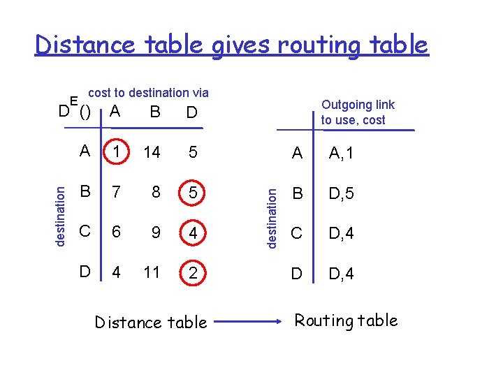
Distance table gives routing table E cost to destination via Outgoing link to use, cost B D A 1 14 5 A A, 1 B 7 8 5 B D, 5 C 6 9 4 C D, 4 D 4 11 2 D D, 4 Distance table destination A destination D () Routing table

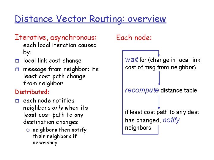
Distance Vector Routing: overview Iterative, asynchronous: each local iteration caused by: r local link cost change r message from neighbor: its least cost path change from neighbor Distributed: r each node notifies neighbors only when its least cost path to any destination changes m neighbors then notify their neighbors if necessary Each node: wait for (change in local link cost of msg from neighbor) recompute distance table if least cost path to any dest has changed, notify neighbors

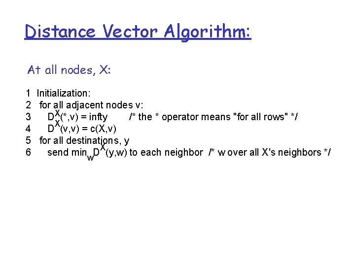
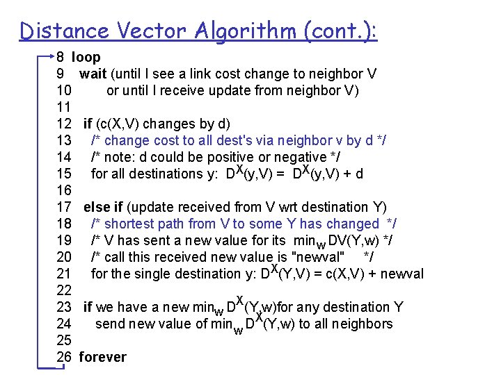
Distance Vector Algorithm: At all nodes, X: 1 Initialization: 2 for all adjacent nodes v: 3 DX(*, v) = infty /* the * operator means "for all rows" */ X 4 D (v, v) = c(X, v) 5 for all destinations, y X 6 send min D (y, w) to each neighbor /* w over all X's neighbors */ w

Distance Vector Algorithm (cont. ): 8 loop 9 wait (until I see a link cost change to neighbor V 10 or until I receive update from neighbor V) 11 12 if (c(X, V) changes by d) 13 /* change cost to all dest's via neighbor v by d */ 14 /* note: d could be positive or negative */ 15 for all destinations y: DX(y, V) = DX(y, V) + d 16 17 else if (update received from V wrt destination Y) 18 /* shortest path from V to some Y has changed */ 19 /* V has sent a new value for its minw DV(Y, w) */ 20 /* call this received new value is "newval" */ 21 for the single destination y: DX(Y, V) = c(X, V) + newval 22 23 if we have a new minw DX(Y, w)for any destination Y 24 send new value of min w DX(Y, w) to all neighbors 25 26 forever

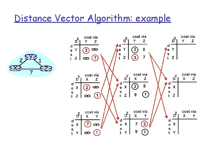
Distance Vector Algorithm: example X 2 Y 7 1 Z

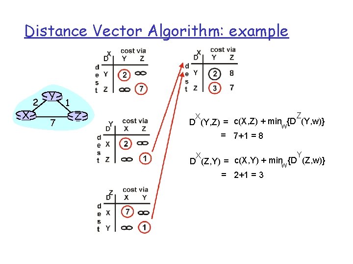
Distance Vector Algorithm: example X 2 Y 7 1 Z Z X D (Y, Z) = c(X, Z) + minw{D (Y, w)} = 7+1 = 8 Y X D (Z, Y) = c(X, Y) + minw {D (Z, w)} = 2+1 = 3

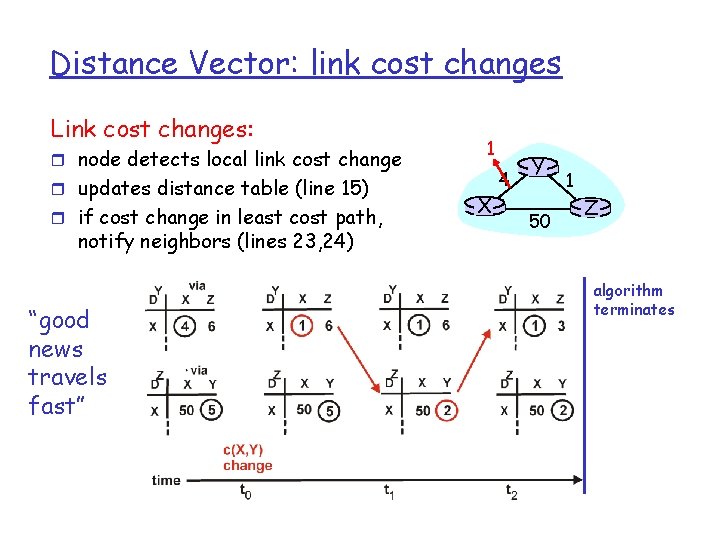
Distance Vector: link cost changes Link cost changes: r node detects local link cost change r updates distance table (line 15) r if cost change in least cost path, notify neighbors (lines 23, 24) “good news travels fast” 1 X 4 Y 50 1 Z algorithm terminates

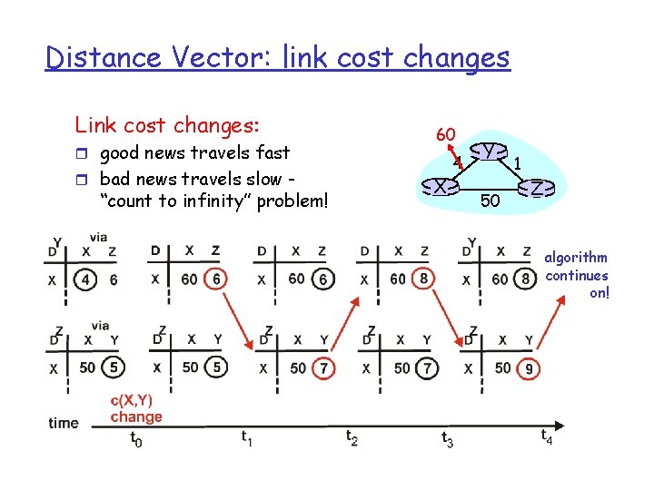
Distance Vector: link cost changes Link cost changes: r good news travels fast r bad news travels slow - “count to infinity” problem! 60 X 4 Y 50 1 Z algorithm continues on!

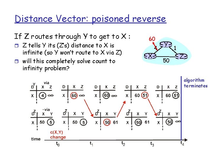
Distance Vector: poisoned reverse If Z routes through Y to get to X : r Z tells Y its (Z’s) distance to X is infinite (so Y won’t route to X via Z) r will this completely solve count to infinity problem? 60 X 4 Y 50 1 Z algorithm terminates

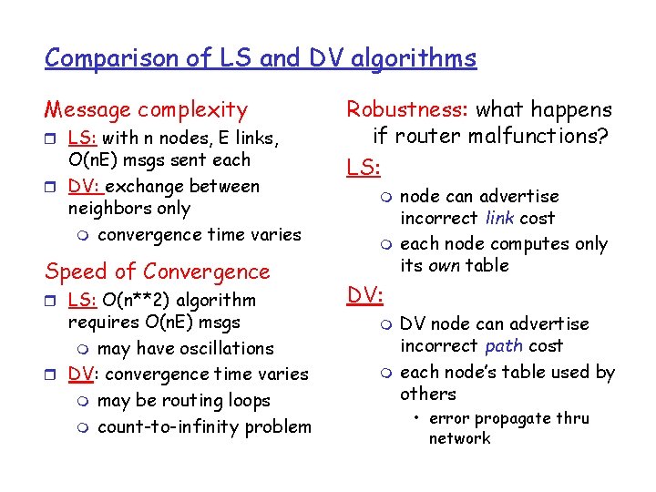
Comparison of LS and DV algorithms Message complexity r LS: with n nodes, E links, O(n. E) msgs sent each r DV: exchange between neighbors only m convergence time varies Speed of Convergence r LS: O(n**2) algorithm requires O(n. E) msgs m may have oscillations r DV: convergence time varies m may be routing loops m count-to-infinity problem Robustness: what happens if router malfunctions? LS: m m node can advertise incorrect link cost each node computes only its own table DV: m m DV node can advertise incorrect path cost each node’s table used by others • error propagate thru network

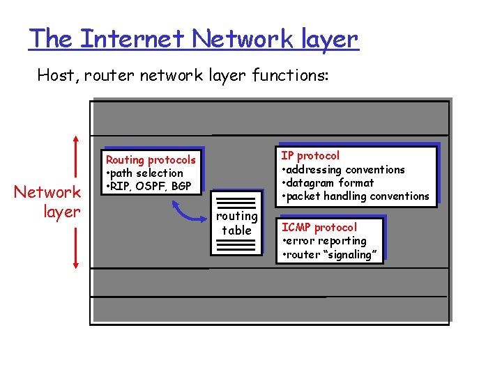
The Internet Network layer Host, router network layer functions: Transport layer: TCP, UDP Network layer IP protocol • addressing conventions • datagram format • packet handling conventions Routing protocols • path selection • RIP, OSPF, BGP routing table ICMP protocol • error reporting • router “signaling” Link layer physical layer