SVY 207 Lecture 11 GPS Error Sources Review

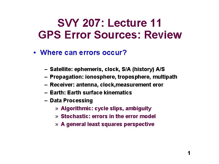
SVY 207: Lecture 11 GPS Error Sources: Review • Where can errors occur? – – – Satellite: ephemeris, clock, S/A (history) A/S Propagation: ionosphere, troposphere, multipath Receiver: antenna, clock, measurement eror Earth: Earth surface kinematics Data Processing » Algorithmic: cycle slips, ambiguity » Stochastic: errors in the error model » A general least squares perspective 1

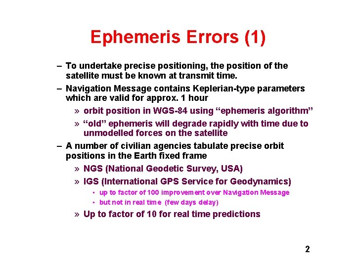
Ephemeris Errors (1) – To undertake precise positioning, the position of the satellite must be known at transmit time. – Navigation Message contains Keplerian-type parameters which are valid for approx. 1 hour » orbit position in WGS-84 using “ephemeris algorithm” » “old” ephemeris will degrade rapidly with time due to unmodelled forces on the satellite – A number of civilian agencies tabulate precise orbit positions in the Earth fixed frame » NGS (National Geodetic Survey, USA) » IGS (International GPS Service for Geodynamics) • up to factor of 100 improvement over Navigation Message • but not in real time (few days delay) » Up to factor of 10 for real time predictions 2

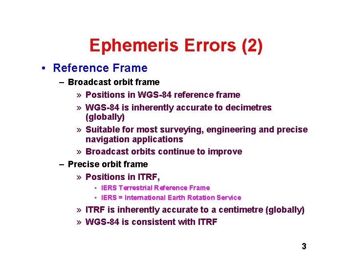
Ephemeris Errors (2) • Reference Frame – Broadcast orbit frame » Positions in WGS-84 reference frame » WGS-84 is inherently accurate to decimetres (globally) » Suitable for most surveying, engineering and precise navigation applications » Broadcast orbits continue to improve – Precise orbit frame » Positions in ITRF, • IERS Terrestrial Reference Frame • IERS = International Earth Rotation Service » ITRF is inherently accurate to a centimetre (globally) » WGS-84 is consistent with ITRF 3

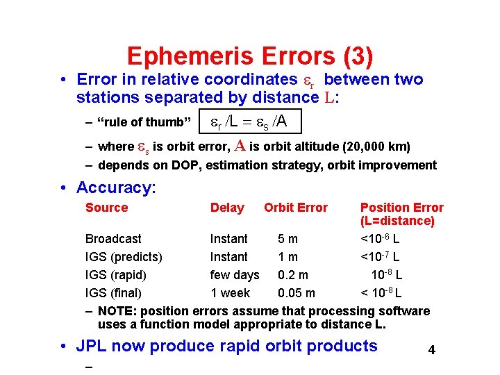
Ephemeris Errors (3) • Error in relative coordinates r between two stations separated by distance L: – “rule of thumb” r L s A – where s is orbit error, A is orbit altitude (20, 000 km) – depends on DOP, estimation strategy, orbit improvement • Accuracy: Source Delay Orbit Error Position Error (L=distance) Broadcast Instant 5 m <10 -6 L IGS (predicts) Instant 1 m <10 -7 L IGS (rapid) few days 0. 2 m 10 -8 L IGS (final) 1 week 0. 05 m < 10 -8 L – NOTE: position errors assume that processing software uses a function model appropriate to distance L. • JPL now produce rapid orbit products – 4

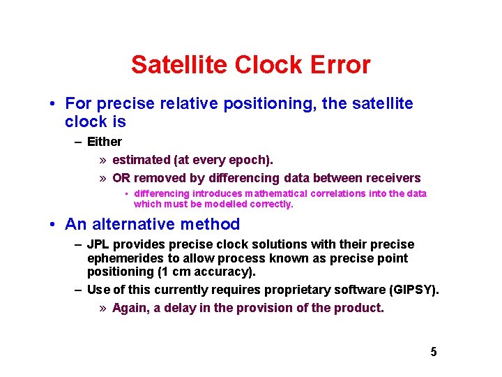
Satellite Clock Error • For precise relative positioning, the satellite clock is – Either » estimated (at every epoch). » OR removed by differencing data between receivers • differencing introduces mathematical correlations into the data which must be modelled correctly. • An alternative method – JPL provides precise clock solutions with their precise ephemerides to allow process known as precise point positioning (1 cm accuracy). – Use of this currently requires proprietary software (GIPSY). » Again, a delay in the provision of the product. 5

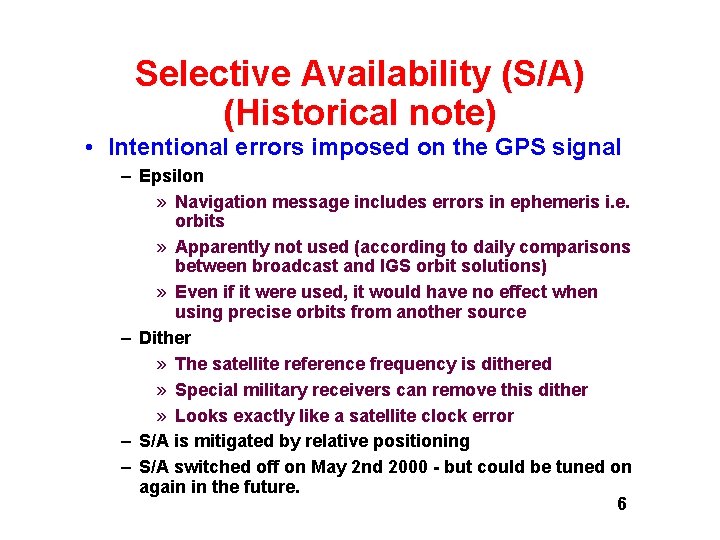
Selective Availability (S/A) (Historical note) • Intentional errors imposed on the GPS signal – Epsilon » Navigation message includes errors in ephemeris i. e. orbits » Apparently not used (according to daily comparisons between broadcast and IGS orbit solutions) » Even if it were used, it would have no effect when using precise orbits from another source – Dither » The satellite reference frequency is dithered » Special military receivers can remove this dither » Looks exactly like a satellite clock error – S/A is mitigated by relative positioning – S/A switched off on May 2 nd 2000 - but could be tuned on again in the future. 6

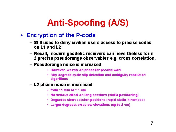
Anti-Spoofing (A/S) • Encryption of the P-code – Still used to deny civilian users access to precise codes on L 1 and L 2 – Recall, modern geodetic receivers can nevertheless form 2 precise pseudorange observables e. g. cross correlation. – Pseudorange noise is increased • However, we rely on phase for precise work • May degrade cycle-slip detection and ambiguity resolution algorithms – L 2 phase noise is increased • • from ~1 mm to ~ 1 cm No serious effect on long sessions (static positioning) Degrades short session positions (rapid static, kinematic) Larger degradation at low elevations (up to 2 cm) 7

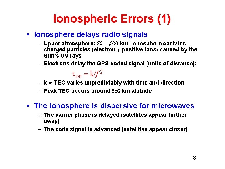
Ionospheric Errors (1) • Ionosphere delays radio signals – Upper atmosphere: km ionosphere contains charged particles (electron positive ions) caused by the Sun’s UV rays – Electrons delay the GPS coded signal (units of distance): ion k f 2 – k TEC varies unpredictably with time and direction – Peak TEC occurs around km altitude • The ionosphere is dispersive for microwaves – The carrier phase is delayed (satellites appear further away) – The code signal is advanced (satellites appear closer) 8

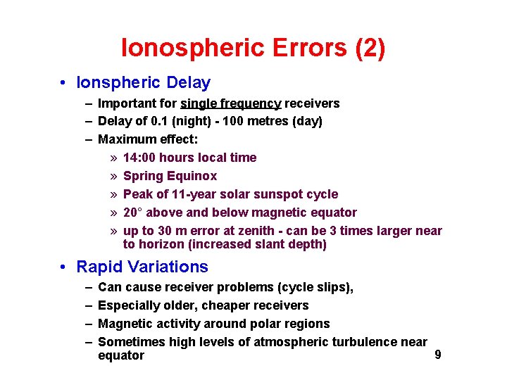
Ionospheric Errors (2) • Ionspheric Delay – Important for single frequency receivers – Delay of 0. 1 (night) - 100 metres (day) – Maximum effect: » 14: 00 hours local time » Spring Equinox » Peak of 11 -year solar sunspot cycle » 20° above and below magnetic equator » up to 30 m error at zenith - can be 3 times larger near to horizon (increased slant depth) • Rapid Variations – – Can cause receiver problems (cycle slips), Especially older, cheaper receivers Magnetic activity around polar regions Sometimes high levels of atmospheric turbulence near 9 equator

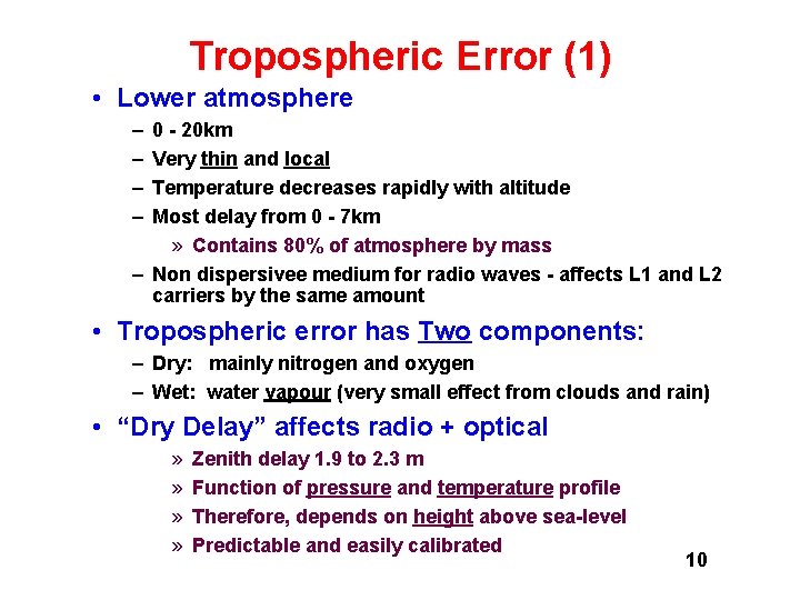
Tropospheric Error (1) • Lower atmosphere – – 0 - 20 km Very thin and local Temperature decreases rapidly with altitude Most delay from 0 - 7 km » Contains 80% of atmosphere by mass – Non dispersivee medium for radio waves - affects L 1 and L 2 carriers by the same amount • Tropospheric error has Two components: – Dry: mainly nitrogen and oxygen – Wet: water vapour (very small effect from clouds and rain) • “Dry Delay” affects radio + optical » » Zenith delay 1. 9 to 2. 3 m Function of pressure and temperature profile Therefore, depends on height above sea-level Predictable and easily calibrated 10

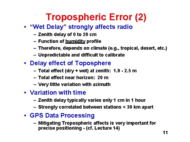
Tropospheric Error (2) • “Wet Delay” strongly affects radio – – Zenith delay of 0 to 20 cm Function of humidity profile Therefore, depends on climate (e. g. , tropical, desert, etc. ) Unpredictable and difficult to calibrate • Delay effect of Toposphere – Total effect (dry + wet) at zenith: 1. 9 - 2. 5 m – Total effect near horizon: 20 m – Very little variation with azimuth • Variation with time – Zenith delay typically varies only 1 cm in 1 hour – Strongly correlated between stations < 30 km apart • GPS Data Processing – Mitigating Tropospheric affects is very important for precise positioning - (cf. Lecture 14) 11

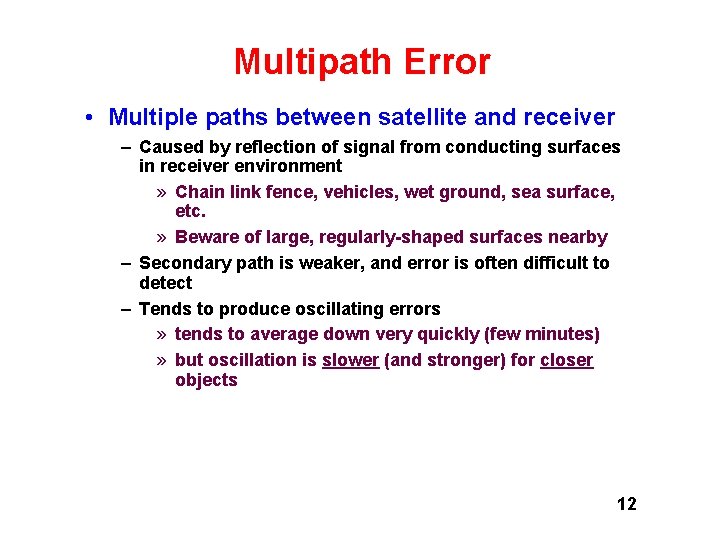
Multipath Error • Multiple paths between satellite and receiver – Caused by reflection of signal from conducting surfaces in receiver environment » Chain link fence, vehicles, wet ground, sea surface, etc. » Beware of large, regularly-shaped surfaces nearby – Secondary path is weaker, and error is often difficult to detect – Tends to produce oscillating errors » tends to average down very quickly (few minutes) » but oscillation is slower (and stronger) for closer objects 12

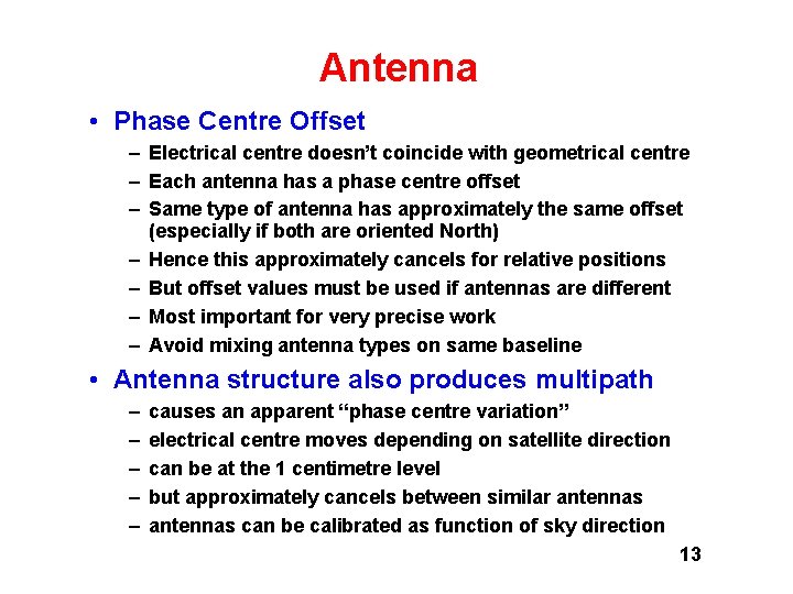
Antenna • Phase Centre Offset – Electrical centre doesn’t coincide with geometrical centre – Each antenna has a phase centre offset – Same type of antenna has approximately the same offset (especially if both are oriented North) – Hence this approximately cancels for relative positions – But offset values must be used if antennas are different – Most important for very precise work – Avoid mixing antenna types on same baseline • Antenna structure also produces multipath – – – causes an apparent “phase centre variation” electrical centre moves depending on satellite direction can be at the 1 centimetre level but approximately cancels between similar antennas can be calibrated as function of sky direction 13

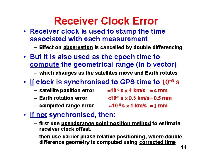
Receiver Clock Error • Receiver clock is used to stamp the time associated with each measurement – Effect on observation is cancelled by double differencing • But it is also used as the epoch time to compute the geometrical range (in b vector) – which changes as the satellites move and Earth rotates • If clock is synchronised to GPS time to s – satellite position error – Earth rotation error – computed range error 10 -6 s 4 km/s mm 10 -6 s 5 km/s mm 10 -6 s 1 km/s mm • If not synchronised, then: – first use pseudorange point position method to estimate receiver clock offset. – then use carrier phase relative positioning, where double difference geometry is computed using corrected time 14

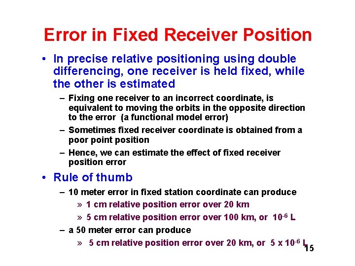
Error in Fixed Receiver Position • In precise relative positioning using double differencing, one receiver is held fixed, while the other is estimated – Fixing one receiver to an incorrect coordinate, is equivalent to moving the orbits in the opposite direction to the error (a functional model error) – Sometimes fixed receiver coordinate is obtained from a poor point position – Hence, we can estimate the effect of fixed receiver position error • Rule of thumb – 10 meter error in fixed station coordinate can produce » 1 cm relative position error over 20 km » 5 cm relative position error over 100 km, or 10 -6 L – a 50 meter error can produce » 5 cm relative position error over 20 km, or 5 x 10 -6 L 15

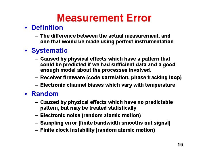
Measurement Error • Definition – The difference between the actual measurement, and one that would be made using perfect instrumentation • Systematic – Caused by physical effects which have a pattern that could be predicted if we had sufficient data and a good enough model about the processes involved. – Receiver firmware (code correlation, phase tracking loop) – Electronic channel biases which vary with temperature • Random – Caused by physical effects which have no predictable pattern, but may be treated statistically – Electronic noise (random atomic motion) – Sampling error (finite bandwidth smooths out signal) – Finite clock instability (random atomic motion) 16

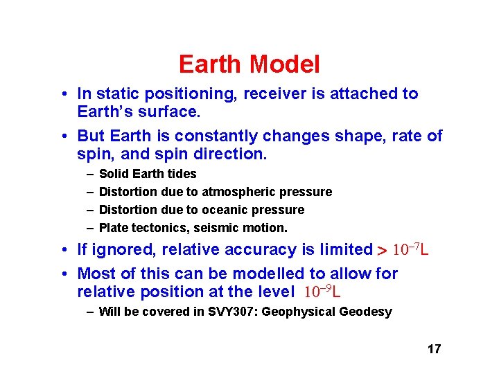
Earth Model • In static positioning, receiver is attached to Earth’s surface. • But Earth is constantly changes shape, rate of spin, and spin direction. – – Solid Earth tides Distortion due to atmospheric pressure Distortion due to oceanic pressure Plate tectonics, seismic motion. • If ignored, relative accuracy is limited L • Most of this can be modelled to allow for relative position at the level L – Will be covered in SVY 307: Geophysical Geodesy 17

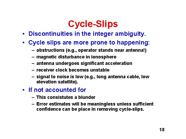
Cycle-Slips • Discontinuities in the integer ambiguity. • Cycle slips are more prone to happening: – – – obstructions (e. g. , operator stands near antenna!) magnetic disturbance in ionosphere antenna undergoes significant acceleration receiver clock becomes unstable signal to noise is low (e. g. , long antenna cable, low elevation satellite). • If not accounted for – This consistutes a blunder – Error estimates will be meaningless unless sufficient confidence can be place in removing cycle-slips. 18

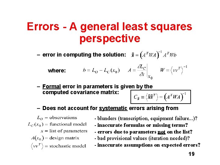
Errors - A general least squares perspective – error in computing the solution: where: – Formal error in parameters is given by the computed covariance matrix: – Does not account for systematic errors arising from - blunders (transcription, equipment failure. . . )? - inaccurate formulas or missing terms? - errors due to parameters not on the list? - bad provisional values (iteration needed)? - inaccurate assumptions on expected errors? 19

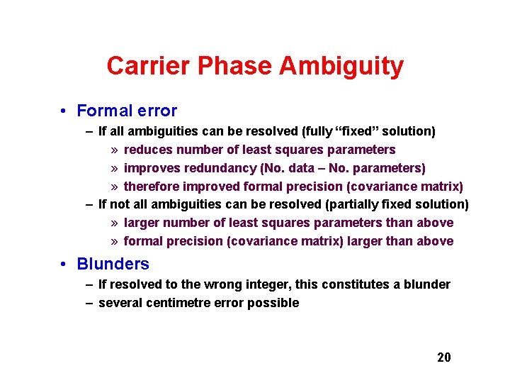
Carrier Phase Ambiguity • Formal error – If all ambiguities can be resolved (fully “fixed” solution) » reduces number of least squares parameters » improves redundancy (No. data No. parameters) » therefore improved formal precision (covariance matrix) – If not all ambiguities can be resolved (partially fixed solution) » larger number of least squares parameters than above » formal precision (covariance matrix) larger than above • Blunders – If resolved to the wrong integer, this constitutes a blunder – several centimetre error possible 20

Stochastic Errors • Finally, it should be recognised that we will introduce an error into our estimates if we have an error in our error model. • Incorrect weight matrix for least-squares – incorrect data variances might be used » low-elevation satellites usually more noisy (low S/N ratio) » In a network solution, we might apply inappropriate weights to a particularly noisy receiver – We might ignore physical correlations between measurements » due to multipath » due to varying atmospheric conditions, etc. » these types of error can equivalently be considered as systematic errors in the functional model. – Software might ignore known mathematical correlations 21