SVM Support Vector Machines A new classification method

SVM - Support Vector Machines • A new classification method for both linear and nonlinear data • It uses a nonlinear mapping to transform the original training data into a higher dimension • With the new dimension, it searches for the linear optimal separating hyperplane (i. e. , “decision boundary”) • With an appropriate nonlinear mapping to a sufficiently high dimension, data from two classes can always be separated by a hyperplane • SVM finds this hyperplane using support vectors (“essential” training tuples) and margins (defined by the support vectors)

SVM - History and Applications • Vapnik and colleagues (1992)—groundwork from Vapnik & Chervonenkis’ statistical learning theory in 1960 s • Features: training can be slow but accuracy is high owing to their ability to model complex nonlinear decision boundaries (margin maximization) • Used both for classification and prediction • Applications: – handwritten digit recognition, object recognition, speaker identification, benchmarking time-series prediction tests

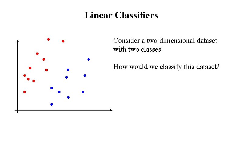
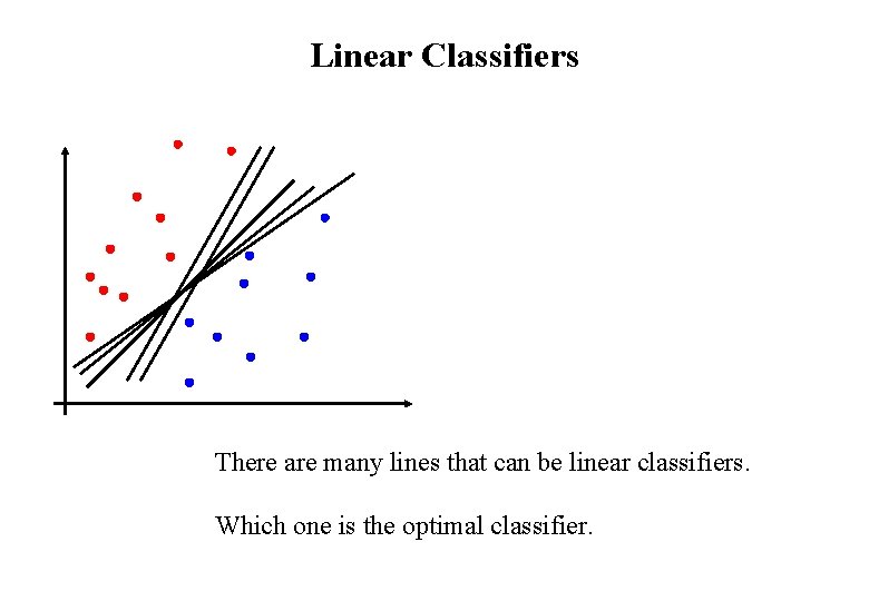
Linear Classifiers Consider a two dimensional dataset with two classes How would we classify this dataset?

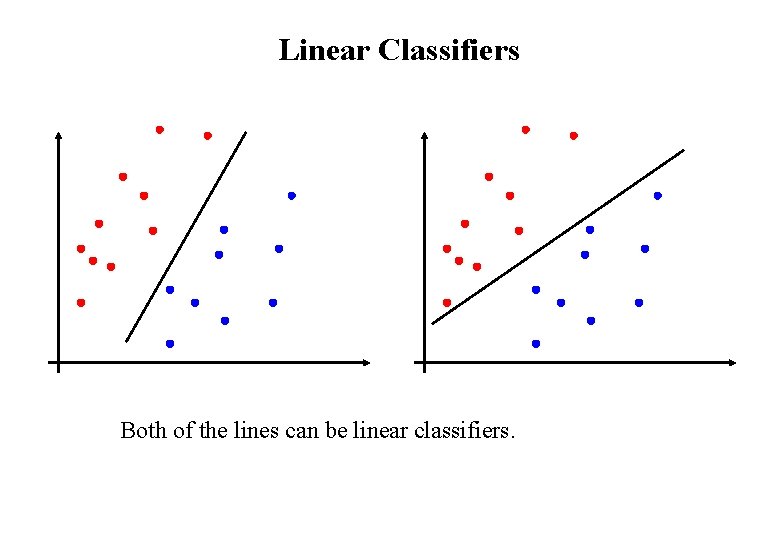
Linear Classifiers Both of the lines can be linear classifiers.

Linear Classifiers There are many lines that can be linear classifiers. Which one is the optimal classifier.

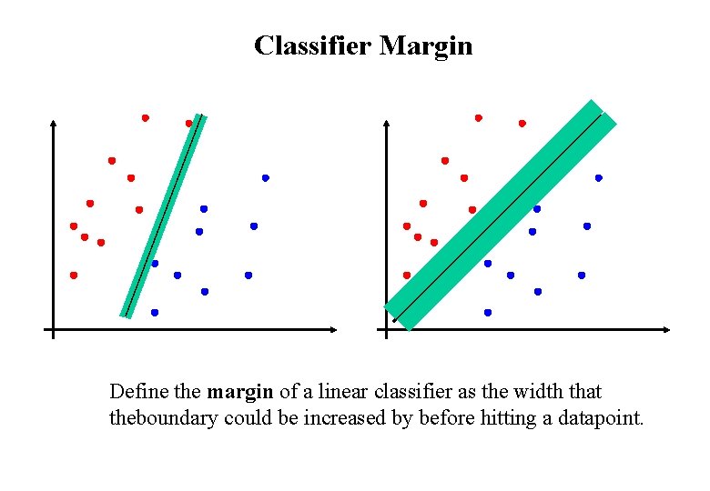
Classifier Margin Define the margin of a linear classifier as the width that theboundary could be increased by before hitting a datapoint.

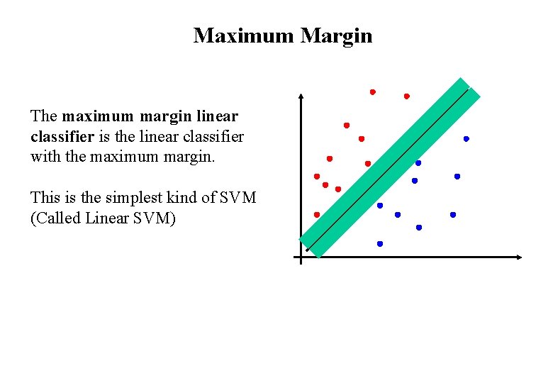
Maximum Margin The maximum margin linear classifier is the linear classifier with the maximum margin. This is the simplest kind of SVM (Called Linear SVM)

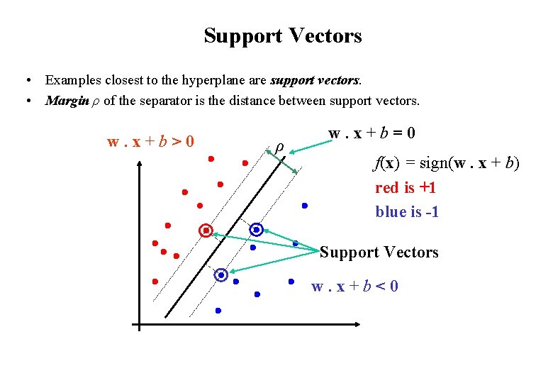
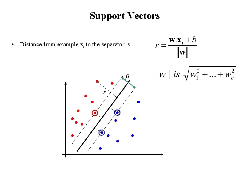
Support Vectors • Examples closest to the hyperplane are support vectors. • Margin ρ of the separator is the distance between support vectors. w. x+b>0 ρ w. x+b=0 f(x) = sign(w. x + b) red is +1 blue is -1 Support Vectors w. x+b<0

Support Vectors • Distance from example xi to the separator is ρ r

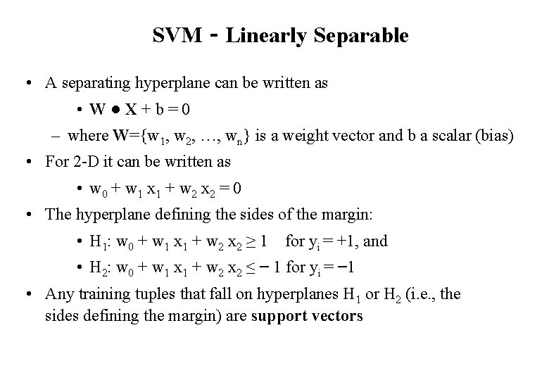
SVM - Linearly Separable • A separating hyperplane can be written as • W●X+b=0 – where W={w 1, w 2, …, wn} is a weight vector and b a scalar (bias) • For 2 -D it can be written as • w 0 + w 1 x 1 + w 2 x 2 = 0 • The hyperplane defining the sides of the margin: • H 1: w 0 + w 1 x 1 + w 2 x 2 ≥ 1 for yi = +1, and • H 2: w 0 + w 1 x 1 + w 2 x 2 ≤ – 1 for yi = – 1 • Any training tuples that fall on hyperplanes H 1 or H 2 (i. e. , the sides defining the margin) are support vectors

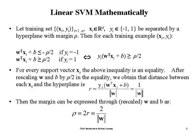
Linear SVM Mathematically • Let training set {(xi, yi)}i=1. . n, xi Rd, yi {-1, 1} be separated by a hyperplane with margin ρ. Then for each training example (xi, yi): w. Txi + b ≤ - ρ/2 if yi = -1 w. Txi + b ≥ ρ/2 if yi = 1 yi(w. Txi + b) ≥ ρ/2 • For every support vector xs the above inequality is an equality. After rescaling w and b by ρ/2 in the equality, we obtain that distance between each xs and the hyperplane is • Then the margin can be expressed through (rescaled) w and b as: CS 464 Introduction to Machine Learning 11

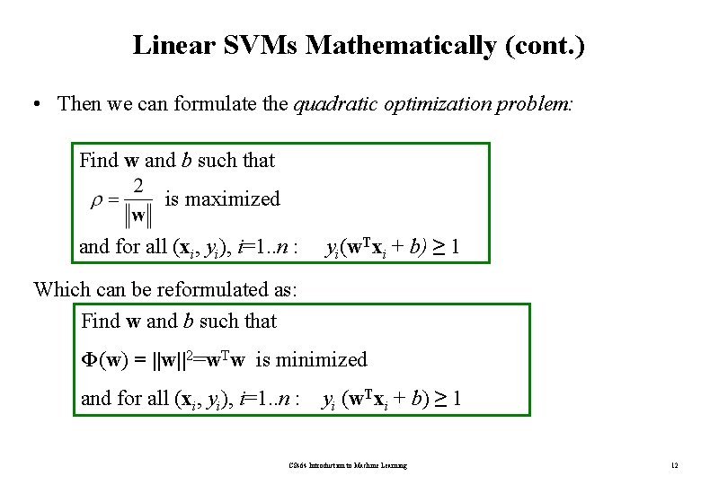
Linear SVMs Mathematically (cont. ) • Then we can formulate the quadratic optimization problem: Find w and b such that is maximized and for all (xi, yi), i=1. . n : yi(w. Txi + b) ≥ 1 Which can be reformulated as: Find w and b such that Φ(w) = ||w||2=w. Tw is minimized and for all (xi, yi), i=1. . n : yi (w. Txi + b) ≥ 1 CS 464 Introduction to Machine Learning 12

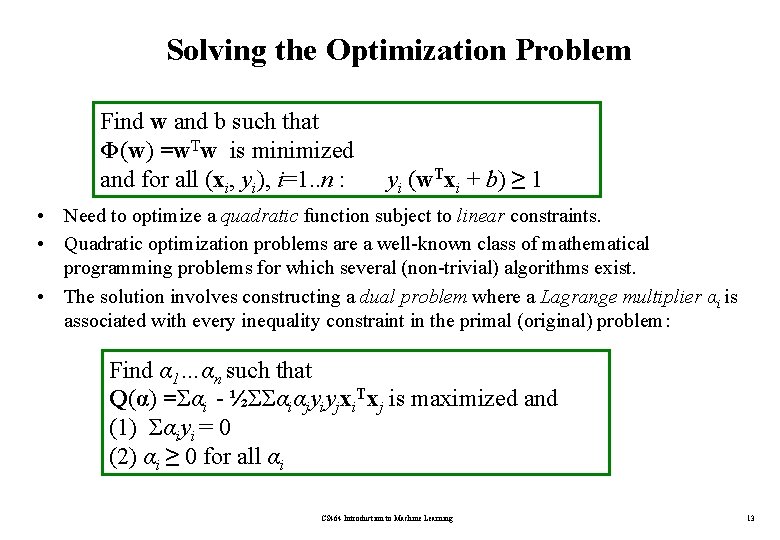
Solving the Optimization Problem Find w and b such that Φ(w) =w. Tw is minimized and for all (xi, yi), i=1. . n : yi (w. Txi + b) ≥ 1 • Need to optimize a quadratic function subject to linear constraints. • Quadratic optimization problems are a well-known class of mathematical programming problems for which several (non-trivial) algorithms exist. • The solution involves constructing a dual problem where a Lagrange multiplier αi is associated with every inequality constraint in the primal (original) problem: Find α 1…αn such that Q(α) =Σαi - ½ΣΣαiαjyiyjxi. Txj is maximized and (1) Σαiyi = 0 (2) αi ≥ 0 for all αi CS 464 Introduction to Machine Learning 13

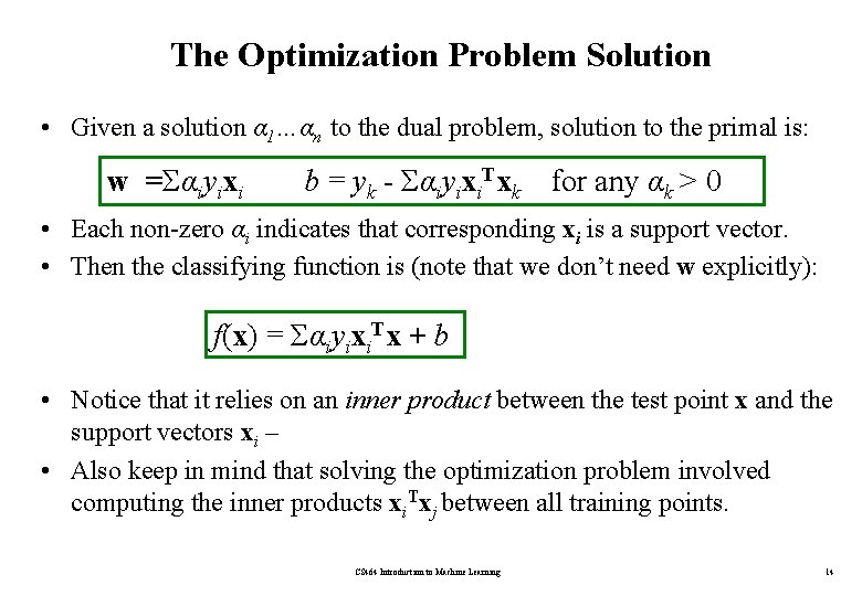
The Optimization Problem Solution • Given a solution α 1…αn to the dual problem, solution to the primal is: w =Σαiyixi b = yk - Σαiyixi. Txk for any αk > 0 • Each non-zero αi indicates that corresponding xi is a support vector. • Then the classifying function is (note that we don’t need w explicitly): f(x) = Σαiyixi. Tx + b • Notice that it relies on an inner product between the test point x and the support vectors xi – • Also keep in mind that solving the optimization problem involved computing the inner products xi. Txj between all training points. CS 464 Introduction to Machine Learning 14

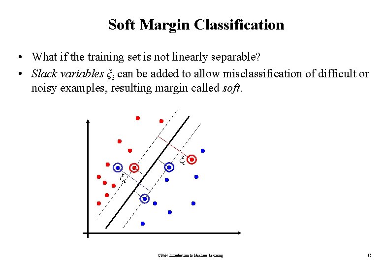
Soft Margin Classification • What if the training set is not linearly separable? • Slack variables ξi can be added to allow misclassification of difficult or noisy examples, resulting margin called soft. ξi ξi CS 464 Introduction to Machine Learning 15

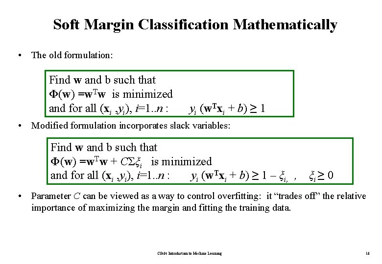
Soft Margin Classification Mathematically • The old formulation: Find w and b such that Φ(w) =w. Tw is minimized and for all (xi , yi), i=1. . n : yi (w. Txi + b) ≥ 1 • Modified formulation incorporates slack variables: Find w and b such that Φ(w) =w. Tw + CΣξi is minimized and for all (xi , yi), i=1. . n : yi (w. Txi + b) ≥ 1 – ξi, , ξi ≥ 0 • Parameter C can be viewed as a way to control overfitting: it “trades off” the relative importance of maximizing the margin and fitting the training data. CS 464 Introduction to Machine Learning 16

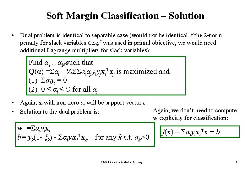
Soft Margin Classification – Solution • Dual problem is identical to separable case (would not be identical if the 2 -norm penalty for slack variables CΣξi 2 was used in primal objective, we would need additional Lagrange multipliers for slack variables): Find α 1…αN such that Q(α) =Σαi - ½ΣΣαiαjyiyjxi. Txj is maximized and (1) Σαiyi = 0 (2) 0 ≤ αi ≤ C for all αi • Again, xi with non-zero αi will be support vectors. • Solution to the dual problem is: w =Σαiyixi b= yk(1 - ξk) - Σαiyixi. Txk for any k s. t. αk>0 CS 464 Introduction to Machine Learning Again, we don’t need to compute w explicitly for classification: f(x) = Σαiyixi. Tx + b 17

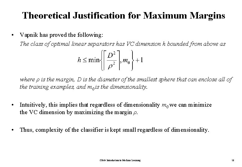
Theoretical Justification for Maximum Margins • Vapnik has proved the following: The class of optimal linear separators has VC dimension h bounded from above as where ρ is the margin, D is the diameter of the smallest sphere that can enclose all of the training examples, and m 0 is the dimensionality. • Intuitively, this implies that regardless of dimensionality m 0 we can minimize the VC dimension by maximizing the margin ρ. • Thus, complexity of the classifier is kept small regardless of dimensionality. CS 464 Introduction to Machine Learning 18

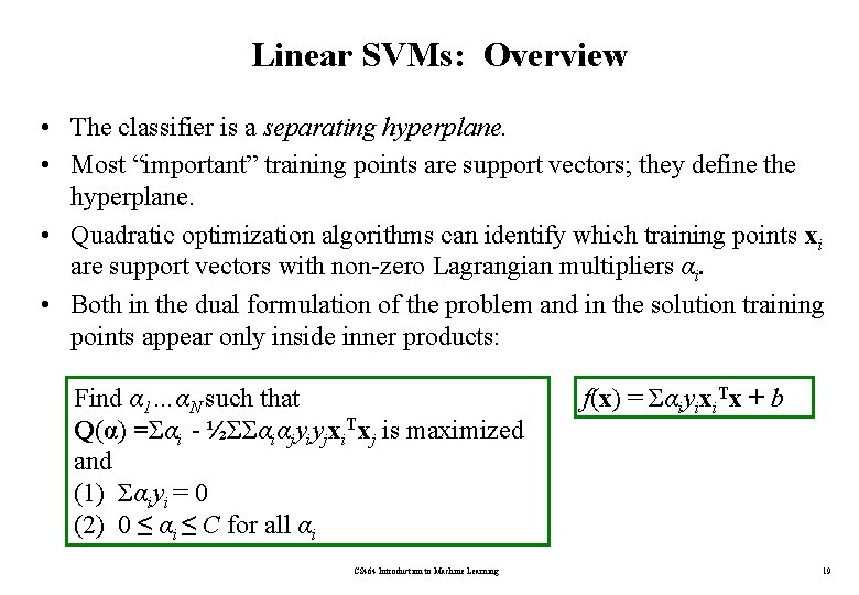
Linear SVMs: Overview • The classifier is a separating hyperplane. • Most “important” training points are support vectors; they define the hyperplane. • Quadratic optimization algorithms can identify which training points xi are support vectors with non-zero Lagrangian multipliers αi. • Both in the dual formulation of the problem and in the solution training points appear only inside inner products: Find α 1…αN such that Q(α) =Σαi - ½ΣΣαiαjyiyjxi. Txj is maximized and (1) Σαiyi = 0 (2) 0 ≤ αi ≤ C for all αi CS 464 Introduction to Machine Learning f(x) = Σαiyixi. Tx + b 19

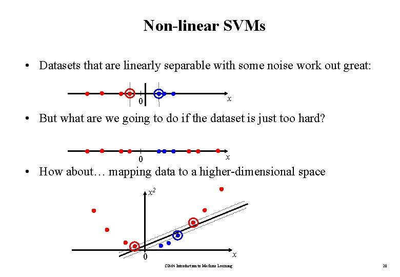
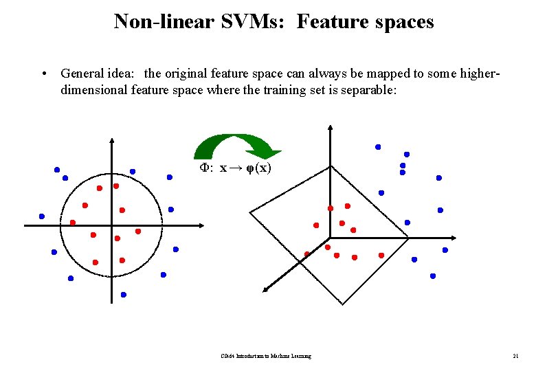
Non-linear SVMs • Datasets that are linearly separable with some noise work out great: x 0 • But what are we going to do if the dataset is just too hard? x 0 • How about… mapping data to a higher-dimensional space x 2 x 0 CS 464 Introduction to Machine Learning 20

Non-linear SVMs: Feature spaces • General idea: the original feature space can always be mapped to some higherdimensional feature space where the training set is separable: Φ: x → φ(x) CS 464 Introduction to Machine Learning 21

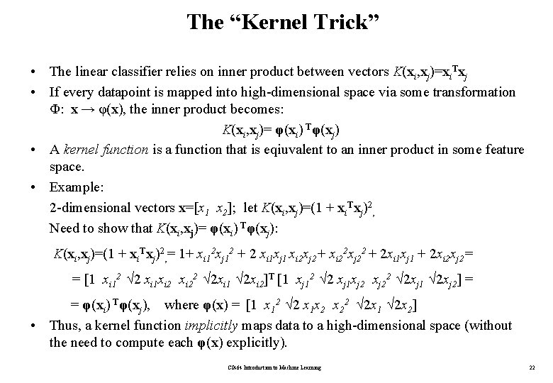
The “Kernel Trick” • The linear classifier relies on inner product between vectors K(xi, xj)=xi. Txj • If every datapoint is mapped into high-dimensional space via some transformation Φ: x → φ(x), the inner product becomes: K(xi, xj)= φ(xi) Tφ(xj) • A kernel function is a function that is eqiuvalent to an inner product in some feature space. • Example: 2 -dimensional vectors x=[x 1 x 2]; let K(xi, xj)=(1 + xi. Txj)2, Need to show that K(xi, xj)= φ(xi) Tφ(xj): K(xi, xj)=(1 + xi. Txj)2, = 1+ xi 12 xj 12 + 2 xi 1 xj 1 xi 2 xj 2+ xi 22 xj 22 + 2 xi 1 xj 1 + 2 xi 2 xj 2= = [1 xi 12 √ 2 xi 1 xi 22 √ 2 xi 1 √ 2 xi 2]T [1 xj 12 √ 2 xj 1 xj 22 √ 2 xj 1 √ 2 xj 2] = = φ(xi) Tφ(xj), where φ(x) = [1 x 12 √ 2 x 1 x 2 x 22 √ 2 x 1 √ 2 x 2] • Thus, a kernel function implicitly maps data to a high-dimensional space (without the need to compute each φ(x) explicitly). CS 464 Introduction to Machine Learning 22

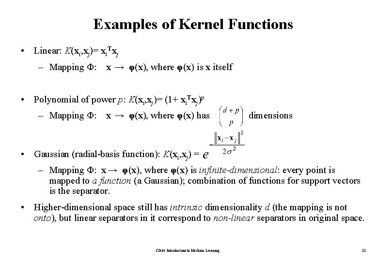
Examples of Kernel Functions • Linear: K(xi, xj)= xi. Txj – Mapping Φ: x → φ(x), where φ(x) is x itself • Polynomial of power p: K(xi, xj)= (1+ xi. Txj)p – Mapping Φ: x → φ(x), where φ(x) has dimensions • Gaussian (radial-basis function): K(xi, xj) = – Mapping Φ: x → φ(x), where φ(x) is infinite-dimensional: every point is mapped to a function (a Gaussian); combination of functions for support vectors is the separator. • Higher-dimensional space still has intrinsic dimensionality d (the mapping is not onto), but linear separators in it correspond to non-linear separators in original space. CS 464 Introduction to Machine Learning 23

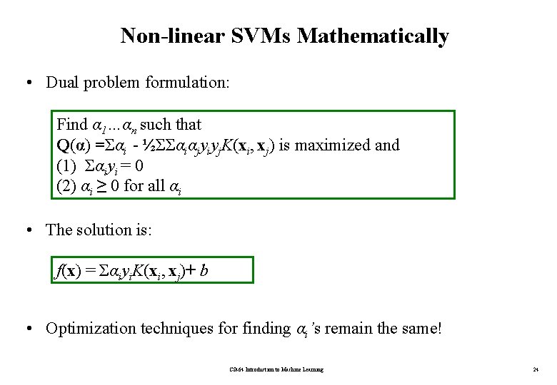
Non-linear SVMs Mathematically • Dual problem formulation: Find α 1…αn such that Q(α) =Σαi - ½ΣΣαiαjyiyj. K(xi, xj) is maximized and (1) Σαiyi = 0 (2) αi ≥ 0 for all αi • The solution is: f(x) = Σαiyi. K(xi, xj)+ b • Optimization techniques for finding αi’s remain the same! CS 464 Introduction to Machine Learning 24

SVM applications • SVMs were originally proposed by Boser, Guyon and Vapnik in 1992 and gained increasing popularity in late 1990 s. • SVMs are currently among the best performers for a number of classification tasks ranging from text to genomic data. • SVMs can be applied to complex data types beyond feature vectors (e. g. graphs, sequences, relational data) by designing kernel functions for such data. • SVM techniques have been extended to a number of tasks such as regression [Vapnik et al. ’ 97], principal component analysis [Schölkopf et al. ’ 99], etc. • Most popular optimization algorithms for SVMs use decomposition to hill-climb over a subset of αi’s at a time, e. g. SMO [Platt ’ 99] and [Joachims ’ 99] • Tuning SVMs remains a black art: selecting a specific kernel and parameters is usually done in a try-and-see manner. CS 464 Introduction to Machine Learning 25