Sustainable Urban Energy Systems A Science of Cities

Sustainable Urban Energy Systems A Science of Cities Approach Lorraine Sugar Ph. D Candidate, University of Toronto ONSEP 2016

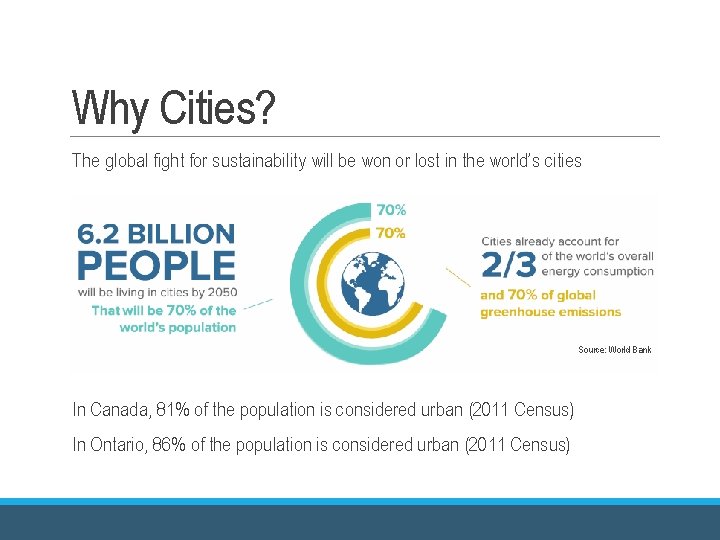
Why Cities? The global fight for sustainability will be won or lost in the world’s cities Source: World Bank In Canada, 81% of the population is considered urban (2011 Census) In Ontario, 86% of the population is considered urban (2011 Census)

The Science of Cities • Rooted in complexity theory • Use principles from physics, mathematics, economics, ecology, etc. to understand cities’ form and function • Main objectives are to develop coherent theories of urban evolution (i. e. , growth and decline) that are descriptive and policy relevant • Theories must • Account for both dynamics and spatial structure • Be empirically testable • Ideally be universally applicable

Properties of Complex Systems • Some properties include: • Feedback loops • Emergent properties, learning, and memory • Order through self-organization, hierarchy, scaling relationships, etc. • Properties observed throughout the natural world (as well as human-made systems!) • Properties can be empirically observed in most complex systems Decoding the Matrix!

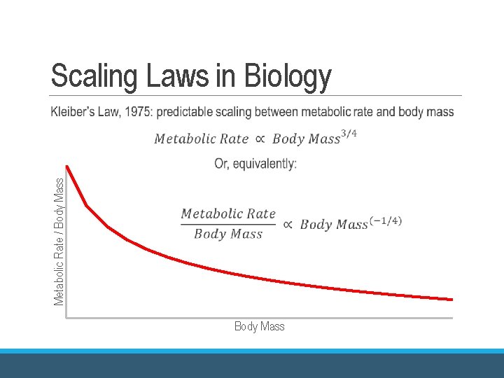
Scaling Laws in Biology Metabolic Rate / Body Mass

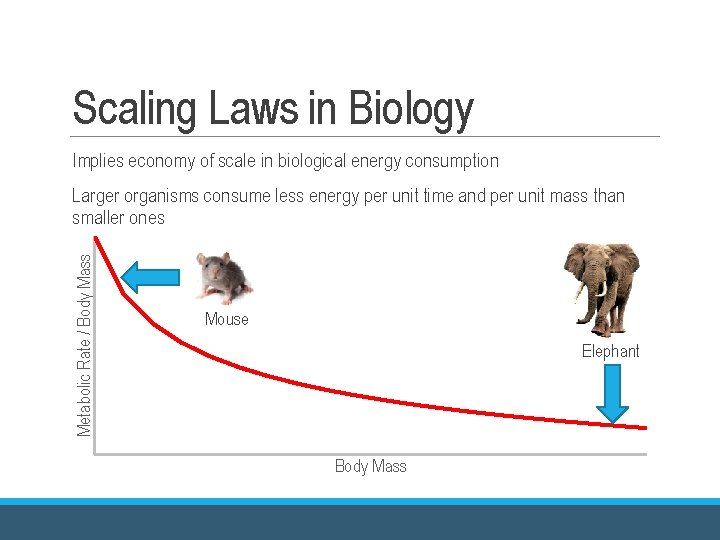
Scaling Laws in Biology Implies economy of scale in biological energy consumption Metabolic Rate / Body Mass Larger organisms consume less energy per unit time and per unit mass than smaller ones Mouse Elephant Body Mass

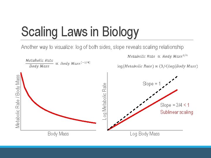
Scaling Laws in Biology Another way to visualize: log of both sides, slope reveals scaling relationship Log Metabolic Rate / Body Mass Slope = 1 Slope = 3/4 < 1 Sublinear scaling Log Body Mass

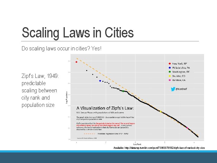
Scaling Laws in Cities Do scaling laws occur in cities? Yes! Zipf’s Law, 1949: predictable scaling between city rank and population size Available: http: //datarep. tumblr. com/post/73860379562/zipfs-law-of-ranked-city-size

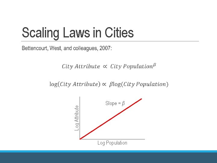
Scaling Laws in Cities Log Attribute Slope = β Log Population

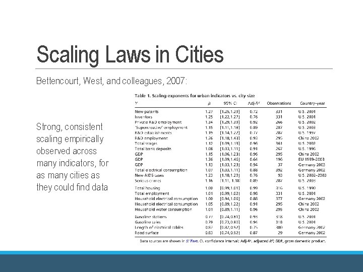
Scaling Laws in Cities Bettencourt, West, and colleagues, 2007: Strong, consistent scaling empirically observed across many indicators, for as many cities as they could find data

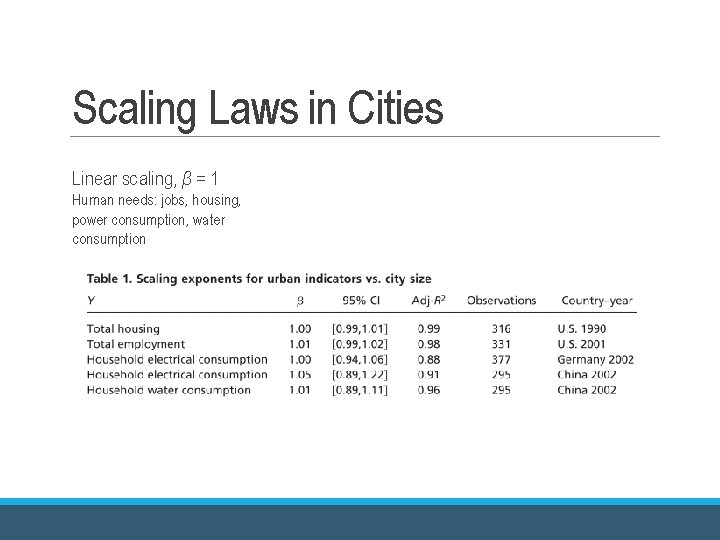
Scaling Laws in Cities Linear scaling, β = 1 Human needs: jobs, housing, power consumption, water consumption

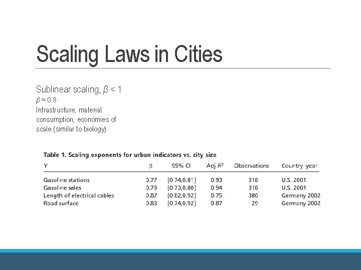
Scaling Laws in Cities Sublinear scaling, β < 1 β ≈ 0. 8 Infrastructure, material consumption, economies of scale (similar to biology)

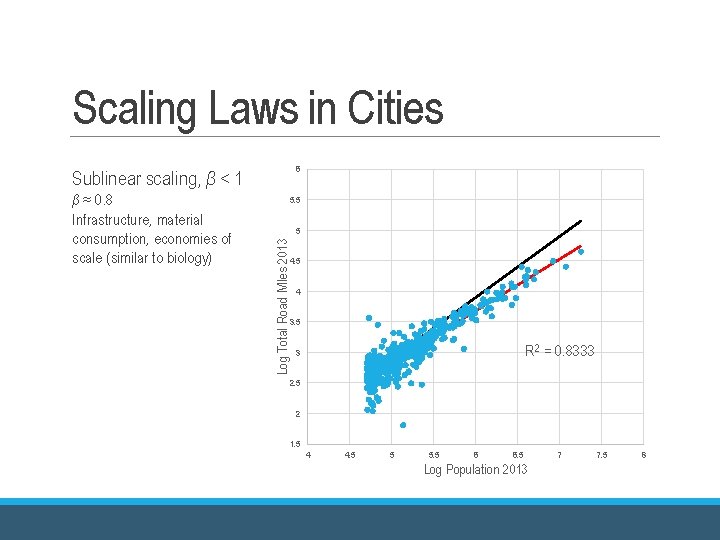
Scaling Laws in Cities 6 Sublinear scaling, β < 1 5. 5 5 Log Total Road Miles 2013 β ≈ 0. 8 Infrastructure, material consumption, economies of scale (similar to biology) 4. 5 4 3. 5 R 2 = 0. 8333 3 2. 5 2 1. 5 4 4. 5 5 5. 5 6 6. 5 Log Population 2013 7 7. 5 8

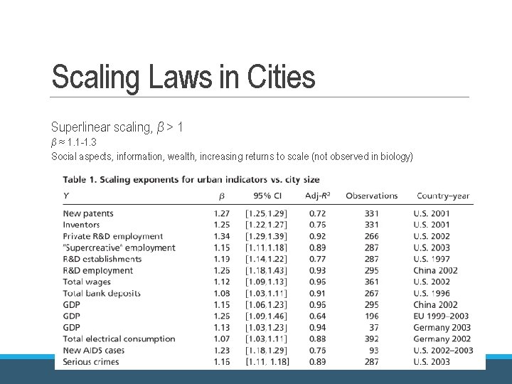
Scaling Laws in Cities Superlinear scaling, β > 1 β ≈ 1. 1 -1. 3 Social aspects, information, wealth, increasing returns to scale (not observed in biology)

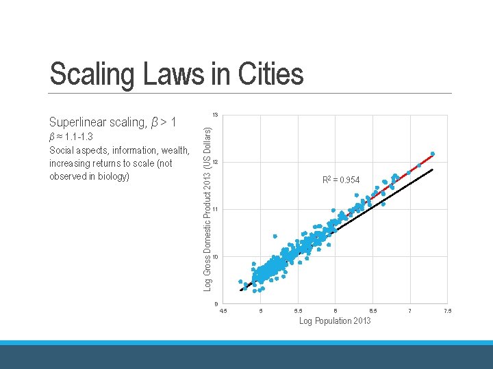
Scaling Laws in Cities β ≈ 1. 1 -1. 3 Social aspects, information, wealth, increasing returns to scale (not observed in biology) Log Gross Domestic Product 2013 (US Dollars) Superlinear scaling, β > 1 13 12 R 2 = 0. 954 11 10 9 4. 5 5 5. 5 6 6. 5 Log Population 2013 7 7. 5

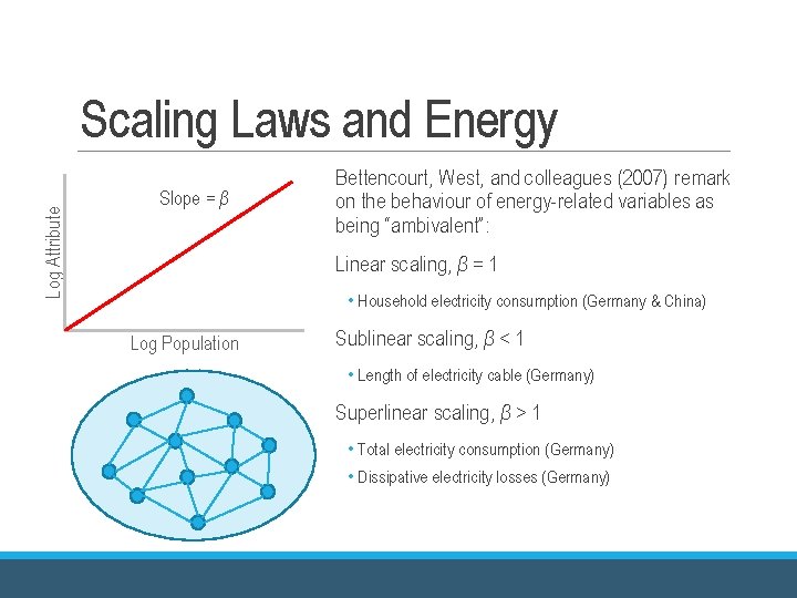
Log Attribute Scaling Laws and Energy Slope = β Bettencourt, West, and colleagues (2007) remark on the behaviour of energy-related variables as being “ambivalent”: Linear scaling, β = 1 • Household electricity consumption (Germany & China) Log Population Sublinear scaling, β < 1 • Length of electricity cable (Germany) Superlinear scaling, β > 1 • Total electricity consumption (Germany) • Dissipative electricity losses (Germany)

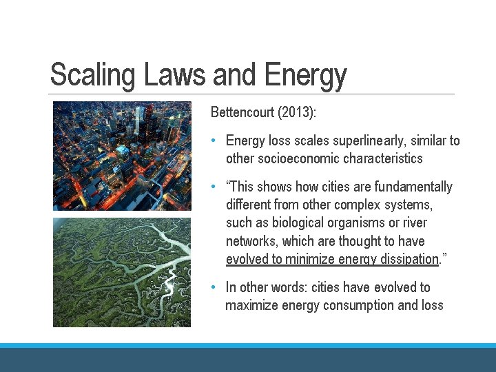
Scaling Laws and Energy Bettencourt (2013): • Energy loss scales superlinearly, similar to other socioeconomic characteristics • “This shows how cities are fundamentally different from other complex systems, such as biological organisms or river networks, which are thought to have evolved to minimize energy dissipation. ” • In other words: cities have evolved to maximize energy consumption and loss

Exploring Policy Relevance • Understanding urban growth • Combining scaling relationships into a helpful parameter, G • Revisiting Kleiber’s Law

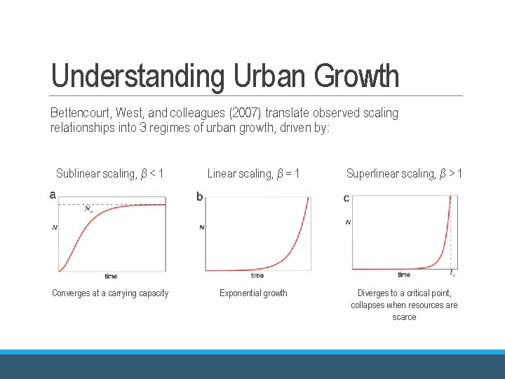
Understanding Urban Growth Bettencourt, West, and colleagues (2007) translate observed scaling relationships into 3 regimes of urban growth, driven by: Sublinear scaling, β < 1 Linear scaling, β = 1 Superlinear scaling, β > 1 Converges at a carrying capacity Exponential growth Diverges to a critical point, collapses when resources are scarce

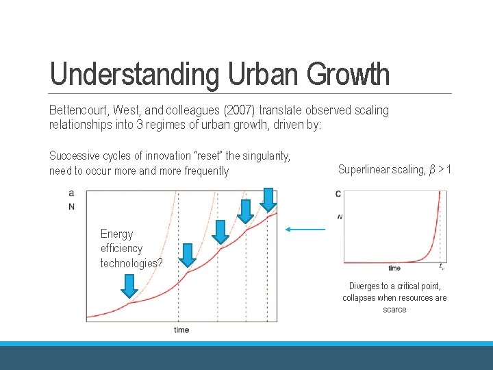
Understanding Urban Growth Bettencourt, West, and colleagues (2007) translate observed scaling relationships into 3 regimes of urban growth, driven by: Successive cycles of innovation “reset” the singularity, need to occur more and more frequently Superlinear scaling, β > 1 Energy efficiency technologies? Diverges to a critical point, collapses when resources are scarce

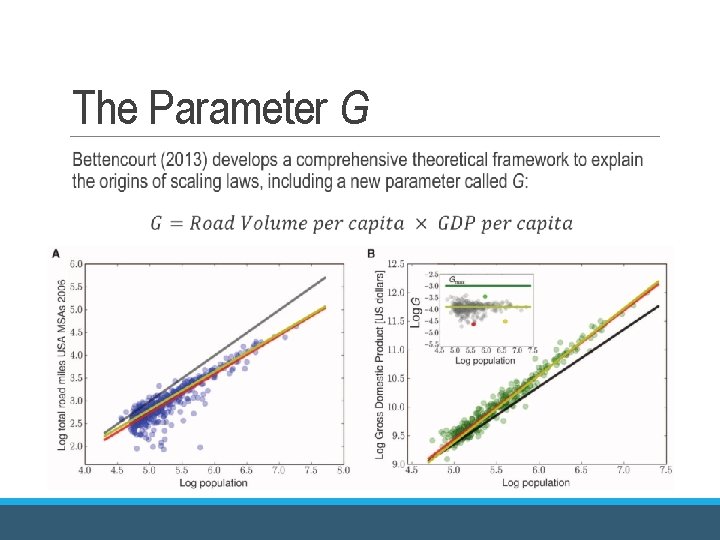
The Parameter G

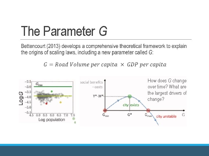
The Parameter G How does G change over time? What are the largest drivers of change?

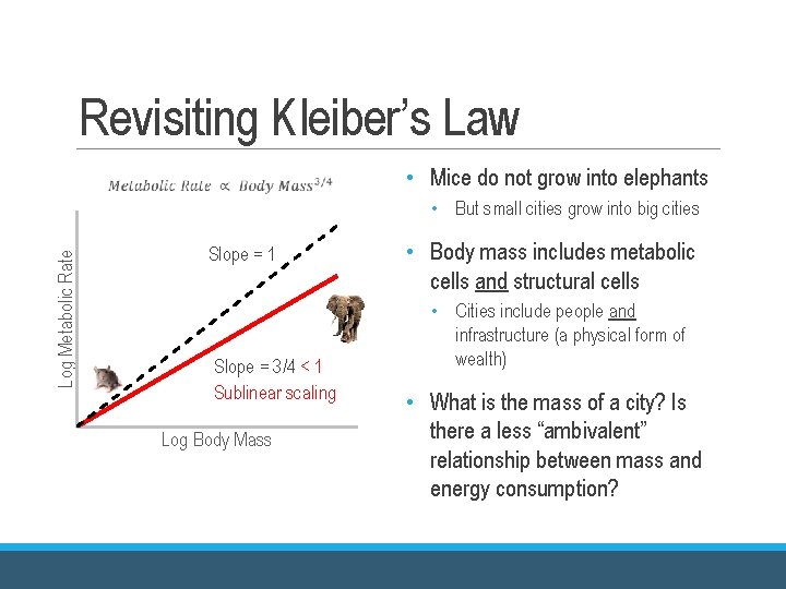
Revisiting Kleiber’s Law • Mice do not grow into elephants Log Metabolic Rate • But small cities grow into big cities Slope = 1 Slope = 3/4 < 1 Sublinear scaling Log Body Mass • Body mass includes metabolic cells and structural cells • Cities include people and infrastructure (a physical form of wealth) • What is the mass of a city? Is there a less “ambivalent” relationship between mass and energy consumption?