Susana Izquierdo Bermudez Rafal Ortwein Juan Carlos Perez

Susana Izquierdo Bermudez, Rafal Ortwein, Juan Carlos Perez, Etienne Rochepault, Nicolas Perey 11 -05 -2016 Overview of ERMC-RMM Magnet Technology Program Acknowledgments: Bernardo Bordini, Paolo Ferracin, Friedrich Lackner, Ezio Todesco, Davide Tommasini, Daniel Schoerling,

Content 1. 2. 3. 4. 5. 6. Introduction Electromagnetic design Mechanical design Engineering design Main technical developments needed Summary and next steps 2

Content 1. 2. 3. 4. 5. 6. Introduction Electromagnetic design Mechanical design Engineering design Main technical developments needed Summary and next steps 3

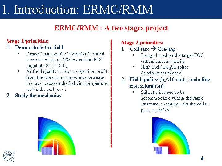
1. Introduction: ERMC/RMM : A two stages project Stage 1 priorities: 1. Demonstrate the field • • Design based on the “available” critical current density (~20% lower than FCC target at 18 T, 4. 2 K) As field quality is not an objective, profit from the use of an iron pole to decrease the ratio between the field in the aperture and in the coil to ~ 1 2. Study the mechanics Stage 2 priorities: 1. Coil size Grading • • Design based on the target FCC critical current density High Field Nb 3 Sn splice development needed 2. Field quality (bn<10 units, including iron saturation) • Still, it will need to be accommodated within the same structure, changing only the collar pack assembly 4

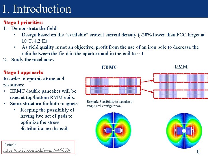
1. Introduction Details: https: //indico. cern. ch/event/446669/ pad pad Stage 1 priorities: 1. Demonstrate the field • Design based on the “available” critical current density (~20% lower than FCC target at 18 T, 4. 2 K) • As field quality is not an objective, profit from the use of an iron pole to decrease the ratio between the field in the aperture and in the coil to ~ 1 2. Study the mechanics RMM ERMC Stage 1 approach: In order to optimise time and resources: • ERMC double pancakes will be used at top/bottom RMM coils. Remark: Possibility to test also a • Same structure for both magnets single coil configuration • Keeping the possibility of having two set of pads to optimize the stress distribution on the coil. 5

1. Introduction Stage 2 priorities: 1. Coil size Grading • • Design based on the target FCC critical current density High Field Nb 3 Sn splice development needed 2. Field quality (bn<10 units, including iron saturation) • Still, it will need to be accommodated within the same structure, changing only the collar pack assembly KEY ISSUE: Development of Nb 3 Sn High field internal splices Strategy: • Magnet design following FCC targets in terms of critical current density and field quality • ERMC will be the base to test the coil technology development: • It should allow the test of a single pancake 6

Content 1. 2. 3. 4. 5. 6. Introduction Electromagnetic design Mechanical design Engineering design Main technical developments needed Summary and next steps 7

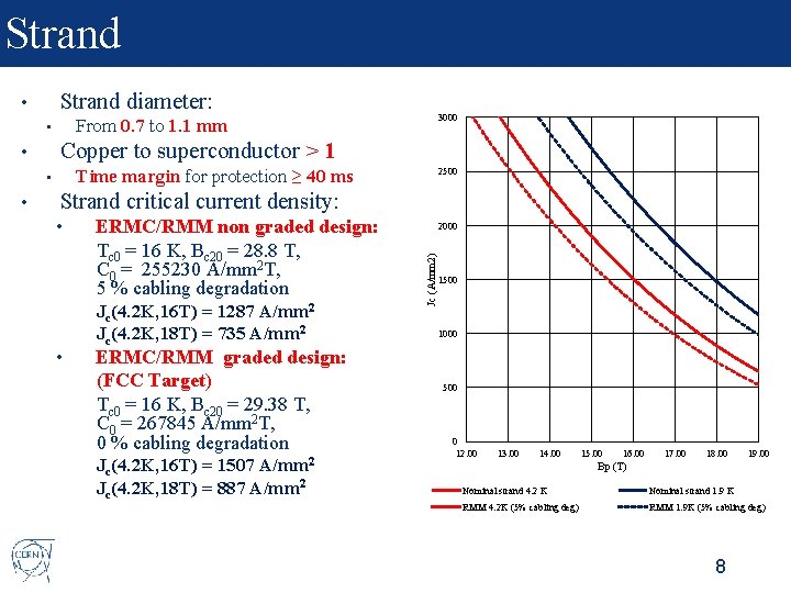
Strand diameter: • Copper to superconductor > 1 Time margin for protection ≥ 40 ms • 2500 Strand critical current density: • • ERMC/RMM non graded design: Tc 0 = 16 K, Bc 20 = 28. 8 T, C 0 = 255230 A/mm 2 T, 5 % cabling degradation Jc(4. 2 K, 16 T) = 1287 A/mm 2 Jc(4. 2 K, 18 T) = 735 A/mm 2 2000 Jc (A/mm 2) • • 3000 From 0. 7 to 1. 1 mm • ERMC/RMM graded design: (FCC Target) Tc 0 = 16 K, Bc 20 = 29. 38 T, C 0 = 267845 A/mm 2 T, 0 % cabling degradation Jc(4. 2 K, 16 T) = 1507 A/mm 2 Jc(4. 2 K, 18 T) = 887 A/mm 2 1500 1000 500 0 12. 00 13. 00 14. 00 15. 00 16. 00 17. 00 18. 00 19. 00 Bp (T) Nominal strand 4. 2 K Nominal strand 1. 9 K RMM 4. 2 K (5% cabling deg) RMM 1. 9 K (5% cabling deg) 8

Cable and Insulation • Non-graded design • • Graded solutions • • 1 mm strand x 40 strands per cable (FRESCA 2) Many options have been explored, decision on what to build has not been taken yet Align with Euro. Cir. Col guidelines to accompany conductor developments needs. Cable insulation thickness = 150 µm • • S 2 -glass/Mica using 11 T development. Parallel material development program to explore and identify enhanced solutions. 9

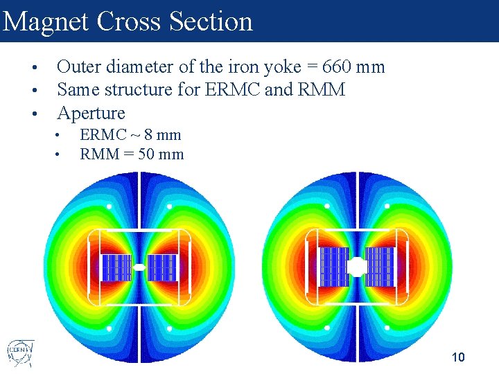
Magnet Cross Section • • • Outer diameter of the iron yoke = 660 mm Same structure for ERMC and RMM Aperture • • ERMC ~ 8 mm RMM = 50 mm 10

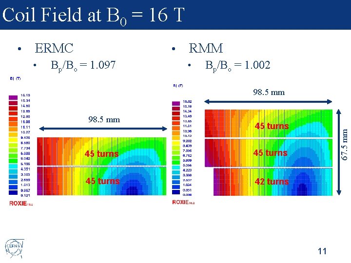
Coil Field at B 0 = 16 T ERMC • • Bp/Bo = 1. 097 RMM • Bp/Bo = 1. 002 98. 5 mm 45 turns 42 turns 67. 5 mm • 11

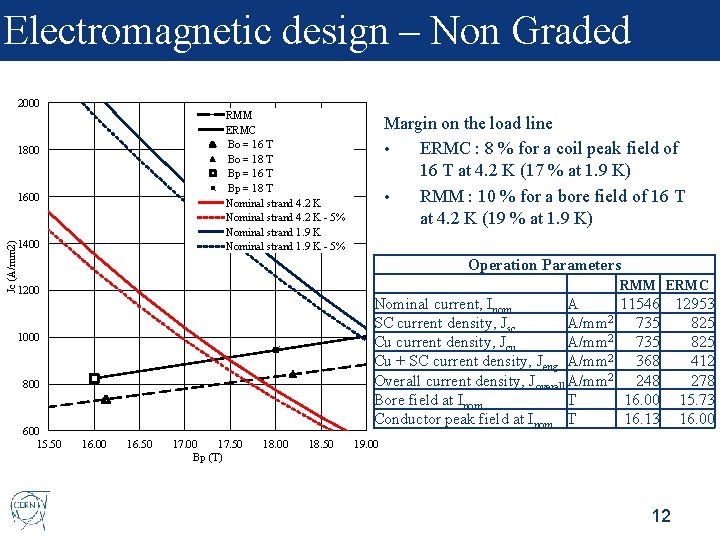
Electromagnetic design – Non Graded 2000 RMM ERMC Bo = 16 T Bo = 18 T Bp = 16 T Bp = 18 T Nominal strand 4. 2 K - 5% Nominal strand 1. 9 K - 5% 1800 Jc (A/mm 2) 1600 1400 Margin on the load line • ERMC : 8 % for a coil peak field of 16 T at 4. 2 K (17 % at 1. 9 K) • RMM : 10 % for a bore field of 16 T at 4. 2 K (19 % at 1. 9 K) Operation Parameters RMM ERMC 1200 Nominal current, Inom A 11546 12953 2 SC current density, Jsc A/mm 735 825 2 Cu current density, Jcu A/mm 735 825 Cu + SC current density, Jeng A/mm 2 368 412 Overall current density, Joverall A/mm 2 248 278 Bore field at Inom T 16. 00 15. 73 Conductor peak field at Inom T 16. 13 16. 00 1000 800 600 15. 50 16. 00 16. 50 17. 00 17. 50 Bp (T) 18. 00 18. 50 19. 00 12

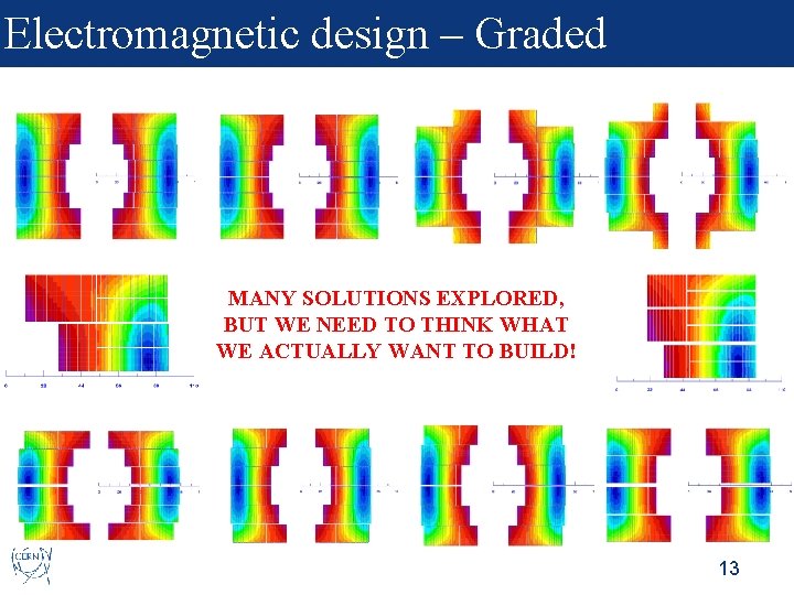
Electromagnetic design – Graded MANY SOLUTIONS EXPLORED, BUT WE NEED TO THINK WHAT WE ACTUALLY WANT TO BUILD! 13

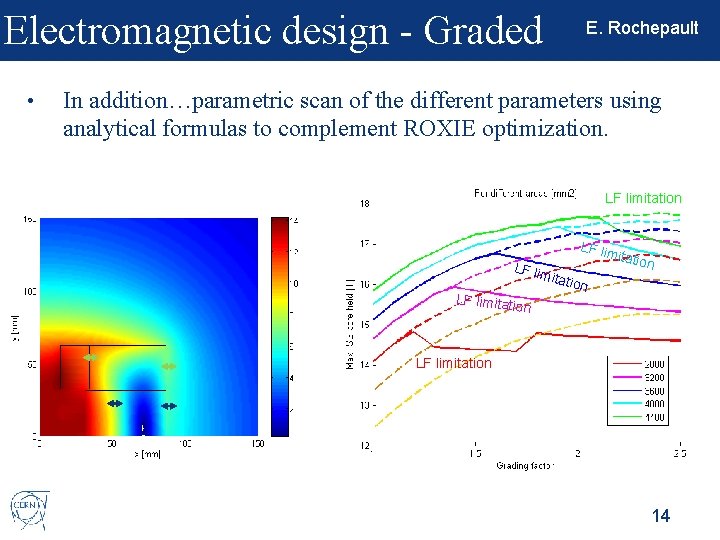
Electromagnetic design - Graded • E. Rochepault In addition…parametric scan of the different parameters using analytical formulas to complement ROXIE optimization. LF limitation LF lim mita tio LF limitatio n n on LF limitation 14

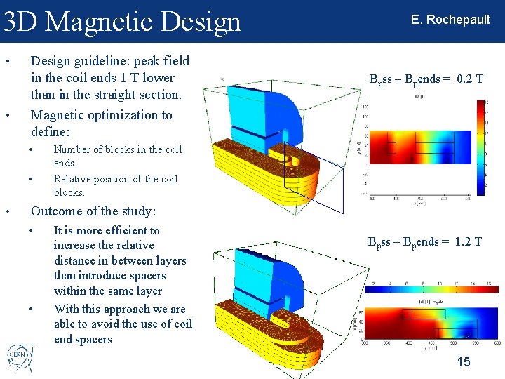
3 D Magnetic Design • • Design guideline: peak field in the coil ends 1 T lower than in the straight section. Magnetic optimization to define: • • • E. Rochepault Bpss – Bpends = 0. 2 T Number of blocks in the coil ends. Relative position of the coil blocks. Outcome of the study: • • It is more efficient to increase the relative distance in between layers than introduce spacers within the same layer With this approach we are able to avoid the use of coil end spacers Bpss – Bpends = 1. 2 T 15

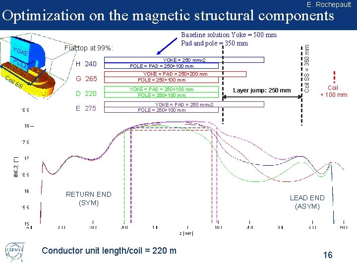
E. Rochepault YOK PO E LE Co il S S Baseline solution Yoke = 500 mm Pad and pole = 350 mm Flat top at 99%: H 240 G 265 D 220 E 275 YOKE = 250 mmx 2 POLE = PAD = 250+100 mm YOKE = PAD = 250+200 mm POLE = 250+100 mm YOKE = PAD = 250+100 mm POLE = 250+100 mm Layer jump: 250 mm Coil SS = 360 mm Optimization on the magnetic structural components Coil + 100 mm YOKE = PAD = 250 mmx 2 POLE = 250+100 mm RETURN END (SYM) Conductor unit length/coil = 220 m LEAD END (ASYM) 16

Content 1. 2. 3. 4. 5. 6. Introduction Electromagnetic design Mechanical design Engineering design Main technical developments needed Summary and next steps 17

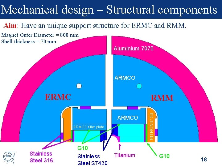
Mechanical design – Structural components Aim: Have an unique support structure for ERMC and RMM. Magnet Outer Diameter = 800 mm Shell thickness = 70 mm Aluminium 7075 ARMCO ERMC ARMCO filler plate Stainless Steel 316: NITRONIC 50 RMM G 10 Stainless Steel ST 430 Titanium G 10 18

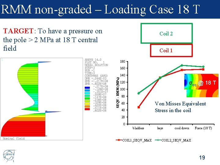
RMM non-graded – Loading Case 18 T TARGET: To have a pressure on the pole > 2 MPa at 18 T central field Coil 2 Coil 1 180 160 SEQV - RMM (MPa) 140 σeq @ 18 T 120 100 80 Von Misses Equivalent Stress in the coil 60 40 20 0 bladders COIL 1_SEQV_MAX keys cool down Force (18 T) COIL 2_SEQV_MAX 19

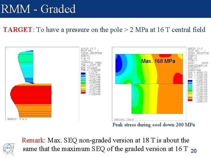
RMM - Graded TARGET: To have a pressure on the pole > 2 MPa at 16 T central field Max. 168 MPa Peak stress during cool down 200 MPa Remark: Max. SEQ non-graded version at 18 T is about the same that the maximum SEQ of the graded version at 16 T 20

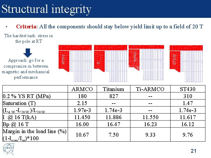
Structural integrity • Criteria: All the components should stay below yield limit up to a field of 20 T ARMCO 0. 2 % YS RT (MPa) 180 Saturation (T) 2. 15 (L 4. 3 K-L 293 K)/L 293 K 1. 97 e-3 I @ 16 T(k. A) 11. 450 Bp @ 16 T 16. 00 Margin in the load line (%) 10. 67 (1 -Inom/Iss)*100 ST 430 armco Ti Approach: go for a compromise in between magnetic and mechanical performance armco The hardest task: stress in the pole at RT Ti Titanium 827 -1. 74 e-3 11. 886 16. 47 Ti-ARMCO ---11. 550 16. 23 ST 430 310 1. 47 1. 74 e-3 11. 617 16. 12 7. 50 9. 33 9. 76 21

3 D Mechanical Design • We just started! 22

Content 1. 2. 3. 4. 5. 6. Introduction Electromagnetic design Mechanical design Engineering design Main technical developments needed Summary and next steps 23

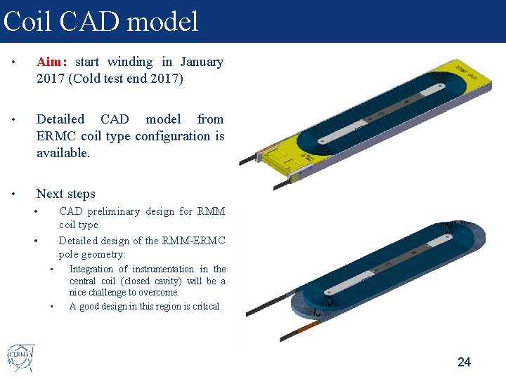
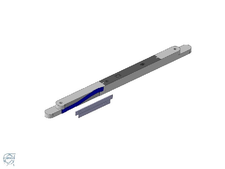
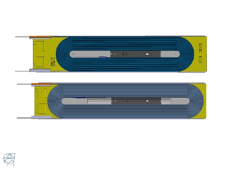
Coil CAD model • Aim: start winding in January 2017 (Cold test end 2017) • Detailed CAD model from ERMC coil type configuration is available. • Next steps CAD preliminary design for RMM coil type Detailed design of the RMM-ERMC pole geometry: • • Integration of instrumentation in the central coil (closed cavity) will be a nice challenge to overcome. A good design in this region is critical. 24

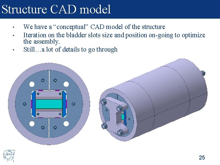
Structure CAD model • • • We have a “conceptual” CAD model of the structure Iteration on the bladder slots size and position on-going to optimize the assembly. Still…a lot of details to go through 25

Content 1. 2. 3. 4. 5. 6. Introduction Electromagnetic design Mechanical design Engineering design Main technical developments needed Summary and next steps 26

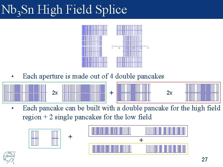
Nb 3 Sn High Field Splice • Each aperture is made out of 4 double pancakes + 2 x • 2 x Each pancake can be built with a double pancake for the high field region + 2 single pancakes for the low field + + 27

Nb 3 Sn High Field Splice • Two possible options: • Winding + Reaction + Splicing + Impregnation • High field and low field are wound together and spliced after reaction • Winding + Reaction + Impregnation + Splicing • High field and low field are wound, reacted and impregnated independently, and they are spliced after impregnation 28

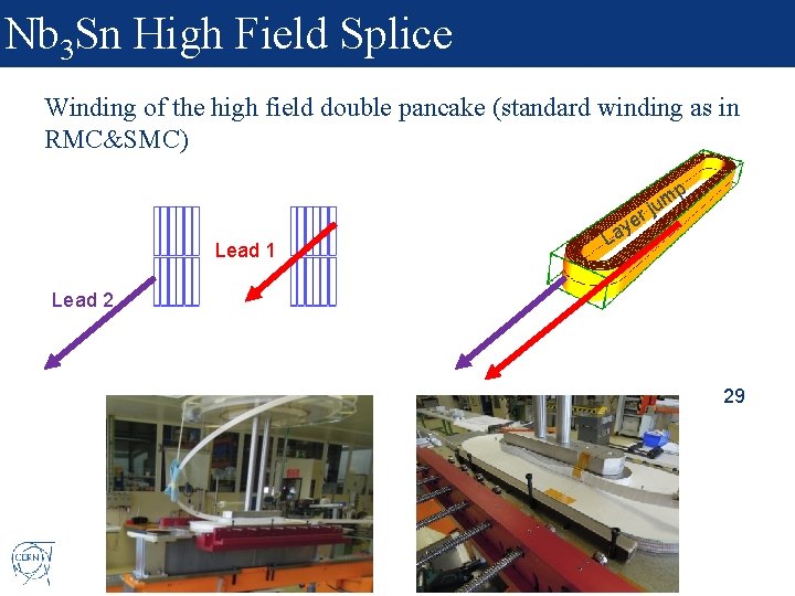
Nb 3 Sn High Field Splice Winding of the high field double pancake (standard winding as in RMC&SMC) r Lead 1 e ay p m ju L Lead 2 29

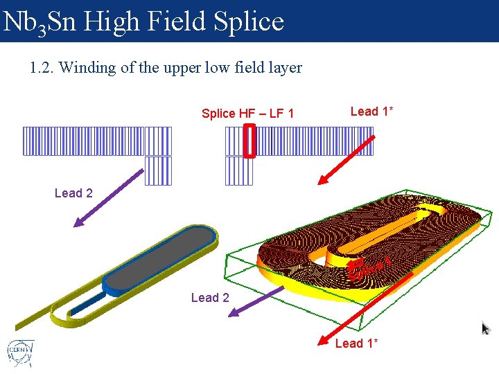
Nb 3 Sn High Field Splice 1. 2. Winding of the upper low field layer Splice HF – LF 1 Lead 1* Lead 2 e plic S Lead 2 Lead 1* 1

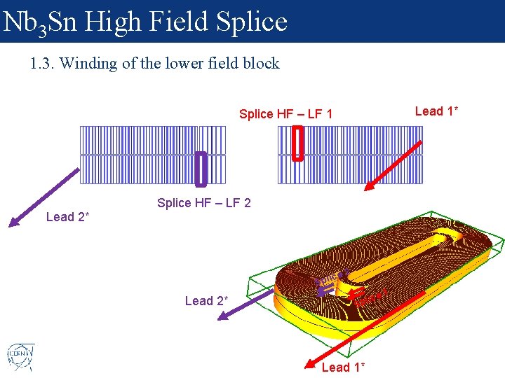
Nb 3 Sn High Field Splice 1. 3. Winding of the lower field block Lead 1* Splice HF – LF 1 Splice HF – LF 2 Lead 2* e 2 ic Spl Lead 2* lice p S Lead 1* 1

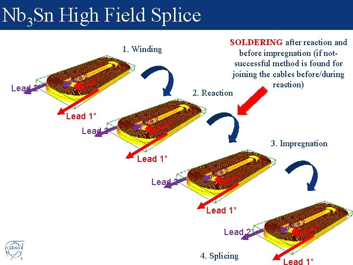
Nb 3 Sn High Field Splice 1. Winding Lead 2* 2 ice ce 1 l p S li Sp Lead 1* Lead 2* SOLDERING after reaction and before impregnation (if notsuccessful method is found for joining the cables before/during reaction) 2. Reaction 2 ice 1 Spl lice p S 3. Impregnation Lead 1* Lead 2* 2 ice l p e 1 S c i l Sp Lead 1* Lead 2* 4. Splicing 2 ice l p e 1 S c i l Sp Lead 1*

Other technical challenges • Winding • • • Insulation • • Based on the 11 T winding experience (0. 7 mm x 40 strands cable, 60 mm aperture), wind-ability in cos-theta configuration for larger cables and smaller aperture should not be underestimated. Coil ends in HD/FRESCA 2 were not optimized in terms of field quality. A coil end optimization including the field quality variable might bring additional complexity that we will need to handle. 11 T cable insulation development pushed forward the electrical integrity of the coil pack, but there is room for optimization. Impregnation • Parallel R&D to understand what are the best materials to put in our coils. ERMC will allow to test the most promising ideas from the parallel R&D programs with a fast turn around time and enough flexibility. 33

Content 1. 2. 3. 4. 5. 6. Introduction Electromagnetic design Mechanical design Engineering design Main technical developments needed Summary and next steps 34

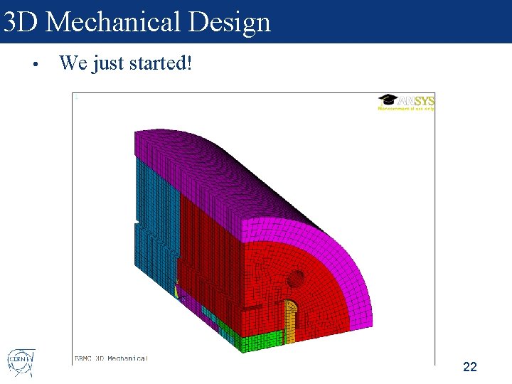
Summary and next steps • We have a stablished program to accompany the 16 T R&D needs in terms of magnet technology development. • First step: Non graded design • • • 2 D design and 3 D magnetic design is done. 3 D mechanical analysis just started. Engineering design is on-going, with the aim of start winding by beginning 2017 (cold test of first ERMC end of 2017). The same structure can be used for a graded coil design with minor modifications. The main challenge is the development of the high field Nb 3 Sn splice. 35

Additional Slides

Contents Parametric study non-graded design 1. Margin on the load line 2. Copper to superconductor ratio 3. Strand diameter 4. Insulation thickness 5. Iron pole 37

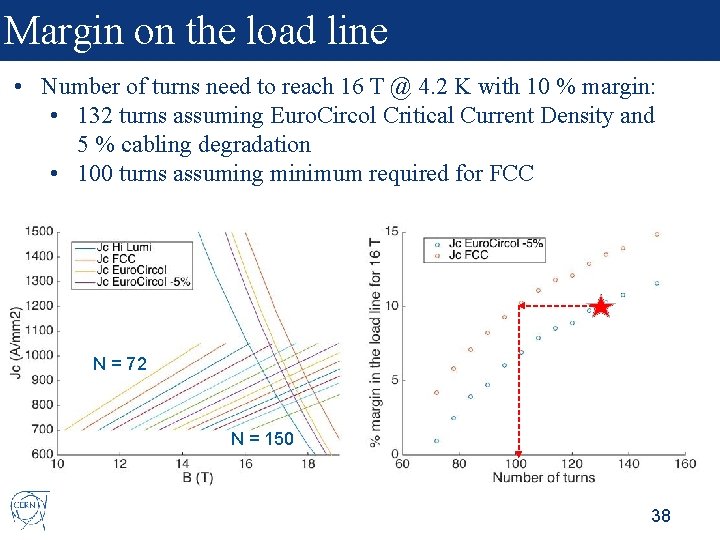
Margin on the load line • Number of turns need to reach 16 T @ 4. 2 K with 10 % margin: • 132 turns assuming Euro. Circol Critical Current Density and 5 % cabling degradation • 100 turns assuming minimum required for FCC N = 72 N = 150 38

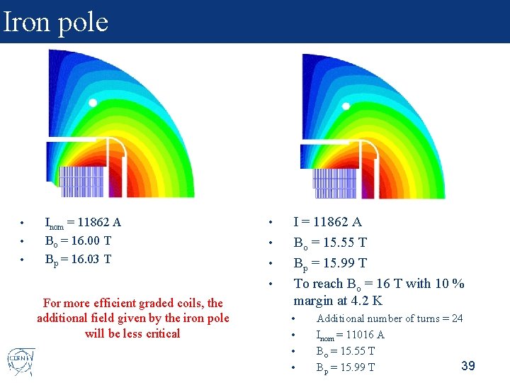
Iron pole • • • Inom = 11862 A Bo = 16. 00 T Bp = 16. 03 T • • For more efficient graded coils, the additional field given by the iron pole will be less critical I = 11862 A Bo = 15. 55 T Bp = 15. 99 T To reach Bo = 16 T with 10 % margin at 4. 2 K • • Additional number of turns = 24 Inom = 11016 A Bo = 15. 55 T 39 Bp = 15. 99 T

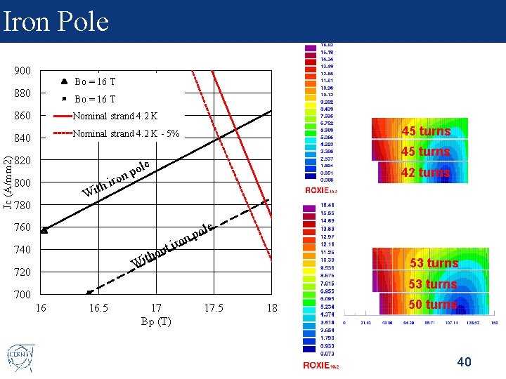
Iron Pole 900 Bo = 16 T Jc (A/mm 2) 880 Bo = 16 T 860 Nominal strand 4. 2 K 840 Nominal strand 4. 2 K - 5% 820 800 t Wi 780 po n o 45 turns le 42 turns h ir ole p on 760 ut o h it 740 ir 53 turns W 720 53 turns 700 16 16. 5 17 Bp (T) 17. 5 18 50 turns 40

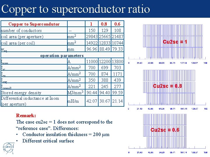
Copper to superconductor ratio Copper to Supercondutor 1 0. 8 0. 6 number of conductors -150 129 108 coil area (per aperture) mm 2 29843 25665 21487 coil area (per coil) mm 2 14922 12833 10744 weq mm 96. 96 88. 49 79. 33 operation parameters Inom A 11000 12200 13800 Jsc A/mm 2 700 699 703 Jcu A/mm 2 700 874 1171 Jeng A/mm 2 350 388 439 Joverall A/mm 2 221 245 277 Stored energy density MJ/mm 3 90. 44 94. 40 99. 59 Differential inductance at Inom m. H/m 42. 07 30. 67 21. 14 (per aperture) Remark: The case cu 2 sc = 1 does not correspond to the “reference case”. Differences: • Conductor insulation thickness = 200 µm • Different critical surface Cu 2 sc = 1 Cu 2 sc = 0. 8 Cu 2 sc = 0. 6 41 41

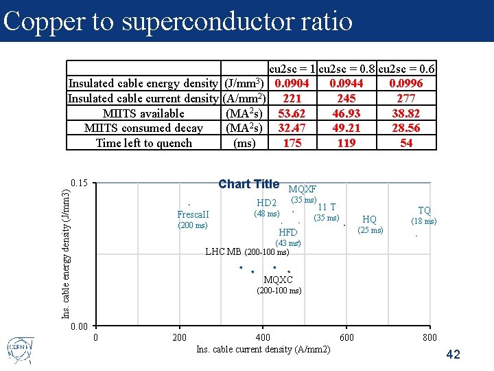
Copper to superconductor ratio cu 2 sc = 1 cu 2 sc = 0. 8 cu 2 sc = 0. 6 Insulated cable energy density (J/mm 3) 0. 0904 0. 0944 0. 0996 Insulated cable current density (A/mm 2) 221 245 277 MIITS available (MA 2 s) 53. 62 46. 93 38. 82 MIITS consumed decay (MA 2 s) 32. 47 49. 21 28. 56 Time left to quench (ms) 175 119 54 Chart Title Ins. cable energy density (J/mm 3) 0. 15 MQXF (35 ms) HD 2 Fresca. II (200 ms) (48 ms) 11 T (35 ms) HFD HQ (25 ms) TQ (18 ms) (43 ms) LHC MB (200 -100 ms) MQXC (200 -100 ms) 0. 00 0 200 400 600 Ins. cable current density (A/mm 2) 800 42

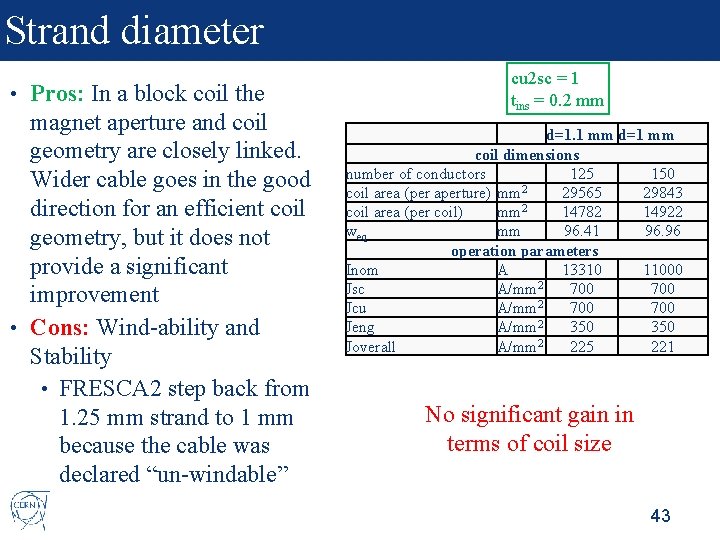
Strand diameter Pros: In a block coil the magnet aperture and coil geometry are closely linked. Wider cable goes in the good direction for an efficient coil geometry, but it does not provide a significant improvement • Cons: Wind-ability and Stability • FRESCA 2 step back from 1. 25 mm strand to 1 mm because the cable was declared “un-windable” • cu 2 sc = 1 tins = 0. 2 mm d=1. 1 mm d=1 mm coil dimensions number of conductors 125 150 coil area (per aperture) mm 2 29565 29843 coil area (per coil) mm 2 14782 14922 weq mm 96. 41 96. 96 operation parameters Inom A 13310 11000 Jsc A/mm 2 700 Jcu A/mm 2 700 2 Jeng A/mm 350 2 Joverall A/mm 225 221 No significant gain in terms of coil size 43

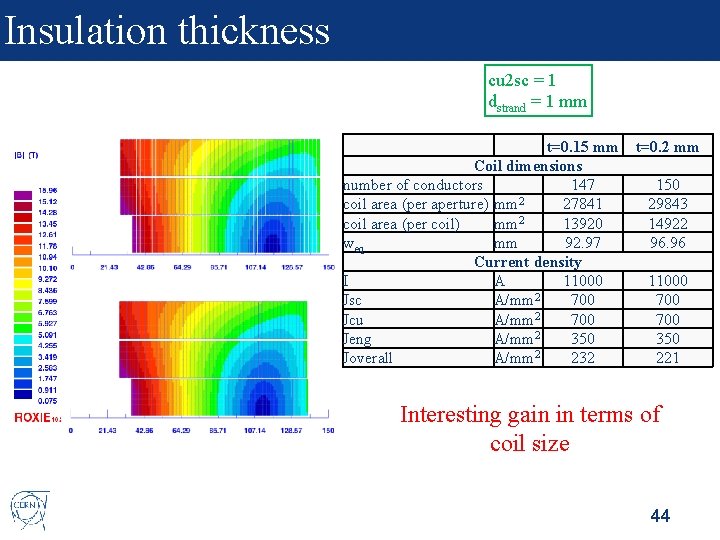
Insulation thickness cu 2 sc = 1 dstrand = 1 mm t=0. 15 mm Coil dimensions number of conductors 147 coil area (per aperture) mm 2 27841 2 coil area (per coil) mm 13920 weq mm 92. 97 Current density I A 11000 Jsc A/mm 2 700 2 Jcu A/mm 700 2 Jeng A/mm 350 Joverall A/mm 2 232 t=0. 2 mm 150 29843 14922 96. 96 11000 700 350 221 Interesting gain in terms of coil size 44