Survival Analysis Gl Ergr RESCAPMed Epi course 22

Survival Analysis Gül Ergör RESCAP-Med Epi course, 22 -26 Sept 2014 Çeşme-Izmir

Outline of Content • What is “Survival Analysis”? Censoring? • How to produce and interpret survival curves? • How to test survival differences between two or more groups of patients? (Comparing Survival Distributions- Log rank test)

Outline of Content • How to quantify survival differences between two or more groups of patients? • How to account for simultaneous influence of a number of explanatory variables? • How to estimate adjusted survival-predictor relationships in the presence of potential confounders (Cox Proportional Hazards Model)

Survival • Time to death from diagnosis is the survival. • Median survival is the time where 50 % of cases are still alive. – Date of diagnosis – Start of therapy – Date of admission to the hospital – Randomisation time in clinical trials

Event • It is not always death – Attack – Relaps – Disease-free survival – Organ rejection

Censored observation • Follow-up ending before the end of the study or before death – Patient wants to leave the study – Lost to follow-up – End of the study

How do we calculate survival time of 10 patients? -Mean? -Median? Person-years? CENSORING MAKES SURVIVAL ANALYSIS DIFFERENT

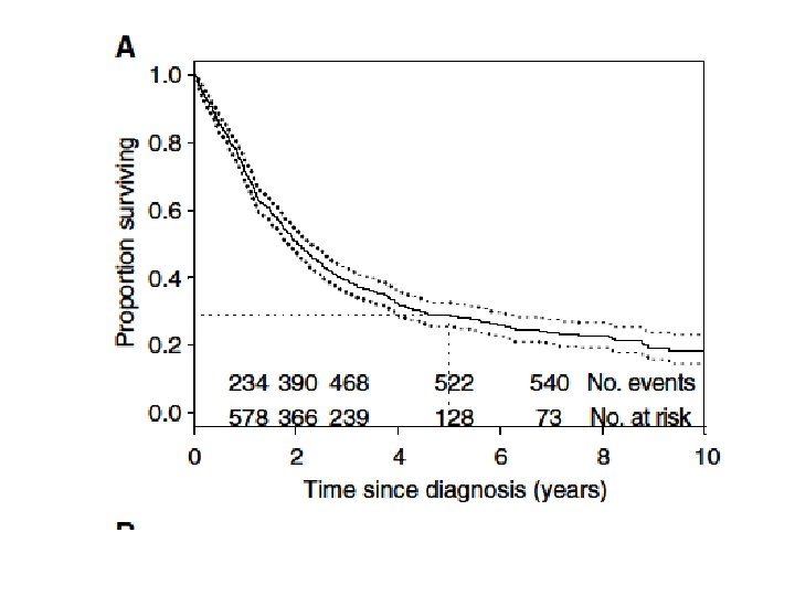
How to produce and interpret survival curves? -Life Table Analysis (Actuarial) -Kaplan Meier Product Limit Estimates of Survival

Kaplan-Meier Method • Time is not divided into intervals • Appropriate for small groups • Survival is calculated when death/event occurs • Censored observations are not taken into account • K-M gives the exact survival probabilities • Survival curve is in steps

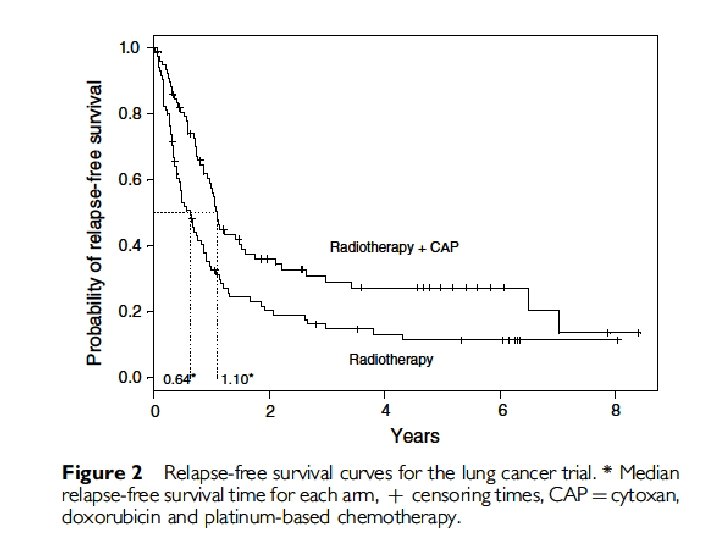
Comparison of two or more Survival Curves • Log-rank test -Gives equal weight to all deaths – Assumes that the ratio of hazard rates in the groups are constant throughout the time period. • The Gehan, or Generalized Wilcoxon test – Attaches more importance to early death

The logrank test statistics is given by This is the same form as the Pearson c 2 test for 2 -way tables! Under the null hypothesis of no difference in survival rates, X 2 will have a chi-square distribution with one degree of freedom. We reject H 0 if X 2 gets too big.

• The Gehan, or Generalized Wilcoxon test -An extension of the Wilcoxon rank-sum test -Every observation in one sample is compared with every observation in the second sample. A mathematical expression involving the ranks is calculated, the function fallows app. z distribution, z distrubition is used statistical significance

Expected number of relapses for each group were 70. 6 and 53. 4, respectively. X 2 =9. 1 (p<0. 002). HR= 0. 58 (there is 42% less risk of relapse at any point in time among patients surviving in the combination treatment group compared with those treated with radiotherapy alone)

logrank test for trend

Cox Proportional Hazard Regression Model • To estimate the magnitude of the survivalpredictor relationship of interest • To account for simultaneous influence of a number of explanatory variables • To estimate adjusted survival-predictor relationships in the presence of potential confounders

Cox Regression Analysis The proportional hazards model In the life table analysis we defined the hazard function as hi = h(ti) = Probability of dying during ith interval given that you survived to the start of the ith interval The instantaneous hazard is just the limiting case of hi as the interval (ti, ti+1) gets very, very small.

Cox Regression Analysis The proportional hazards model So let h(t|X 1, X 2, …, Xk) = probability of “dying” on day t given survival up to day t and baseline covariates X 1, X 2, …, Xk define the instantaneous hazard at time t. The Cox proportional hazards model assumes that h(t) can be written as β is the logarithm of the hazard Rates Ratio (R. R. )

Cox P H Regression Model. Assumptions • Key assumption of the Cox model is proportional hazards • The hazard ratio will remain constant over time • But not the same over time

Cox P H Regression Model. Assumptions • Smokers Hazard Smokers Constant Ratio Time Never. Smokers 23

Cox P H Regression- Formula h(t, X) = ho(t) e β 0 + β 1 X 1 + β 2 X 2 ho(t) baseline h involves t but not X’s X e∑ βi Xi exponential involves X’s but not t 24

Cox P H Regression h(t, X) = ho(t) eβ 1 X 1 + β 2 X 2 If X’s = 0, then h(t, X)= h 0(t) e 0 = h 0(t) 1 h(t, X)= h 0(t) the baseline function 25

Cox P H Regression – A Simple Example Data • T= Diagnosis to death (in months) (1) • 300 lung cancer patients – Gender • Female group (1) • Male Group (0) – Age 26

Cox P H Regression – A Simple Example Question What is the association between death and being female, adjusting for age? Comparing the survival of the two groups adjusting for possible confounding effect of age. 27

Cox P H Regression- output Variables in the Equation B SE Wald df Sig. Exp(B) 95% CI for Exp(B) Lower Upper Gender -. 484 . 237 -2. 05 1 0. 041 0. 616 0. 388 0, 979 Age yr 0, 040 . 009 4. 54 1 , 000 1. 041 1, 023 1, 059 28

Cox P H Regression – A Simple Example ho(t) eβ 1 age + β 2 female RR (female vs male) = = ho(t) eβ 1 age + β 2 h o(t) eβ 1 age eβ 2 => β 2 = ln(RRmales vs females) 29

Cox PH- Interpretation �� β 1 > 0 : Higher hazard (poorer survival) associated with being female �� Because e β 1 > 1 β 1 < 0 : Lower hazard (better survival) associated with being female �� Because e β 1 < 1 30

Cox P H Regression- categorical • B SE Wald df Sig. Exp(B) 95% CI for Exp(B) Lower Gender Age yr Upper -. 484 . 237 -2. 05 1 0. 041 0. 616 0. 388 0, 979 0, 040 . 009 4. 54 1 , 000 1. 041 1, 023 1, 059 31

Cox P H Regression- categorical Interpretation B SE Wald df Sig. Exp(B) 95% CI for Exp(B) Lower Upper Gender -. 484 . 237 -2. 05 1 0. 041 0. 616 0. 388 0, 979 Age yr 0, 040 . 009 4. 54 1 , 000 1. 041 1, 023 1, 059 After adjusting for age the estimate hazard ratio (relative risk) of death for females compared to males is e -. 48 =. 62 Females have. 62 the hazard (risk) that males have of death, after aged-adjusted. Females have 38% lower hazard (risk) of death than males, after age-adjusted. 32

Cox P H Regression- categorical Interpretation • In a sample of 300 NSCLC patients, females had a lower hazard (risk) of death than males, after age-adjusted. The estimated hazard ratio was. 62 indicating that females had 38% lower hazard (risk) of death than males. • Accounting for sampling variability, the decrease in risk for females could be as large as 62% or as small as 3% (95% CI for the hazard ratio 0. 38 – 0. 97). 33

Cox P H Regression- continuous B SE Wald df Sig. Exp(B) 95% CI for Exp(B) Lower Upper Gender -. 484 . 237 -2. 05 1 0. 041 0. 616 0. 388 0, 979 Age yr 0, 040 . 009 4. 54 1 , 000 1. 041 1, 023 1, 059 In this sample, after gender-adjusted, a one-year increase in age is associated with a 4% increase in the hazard (risk) of death. In other words, if we were to compare two groups of persons who differ by one year in age, the older group has a 4% higher risk of death than the younger group 34