Survival analysis Brian Healy Ph D Previous classes

Survival analysis Brian Healy, Ph. D

Previous classes n Regression – Linear regression – Multiple regression – Logistic regression

What are we doing today? n Survival analysis – Kaplan-Meier curve – Dichotomous predictor – How to interpret results n Cox proportional hazards – Continuous predictor – How to interpret results

Big picture n In medical research, we often confront continuous, ordinal or dichotomous outcomes n One other common outcome is time to event (survival time) – Clinical trials often measure time to death or time to relapse n We would like to estimate the survival distribution

Types of analysis-independent samples Outcome Explanatory Analysis Continuous Dichotomous t-test, Wilcoxon test Continuous Categorical ANOVA, linear regression Continuous Dichotomous Continuous Correlation, linear regression Chi-square test, logistic regression Logistic regression Time to event Dichotomous Log-rank test

Definitions n Survival time: time to event n Survival function: probability survival time is greater than a specific value S(t)=P(T>t) n Hazard function: risk of having the event l(t)=# who had event/# at risk n These two factors are mathematically related

Example n An important marker of disease activity in MS is the occurrence of a relapse – This is the presence of new symptoms that lasts for at least 24 hours n Many clinical trials in MS have demonstrated that treatments increase the time until the next relapse – How does the time to next relapse look in the clinic? n What is the distribution of survival times?

Kaplan-Meier curve Each drop in the curve represents an event

Survival data n To create this curve, patients placed on treatment were followed and the time of the first relapse on treatment was recorded – Survival time If everyone had an event, some of the methods we have already learned could be applied n Often, not everyone has event n – Loss to follow-up – End of study

Censoring n The patients who did not have the event are considered censored – We know that they survived a specific amount of time, but do not know the exact time of the event – We believe that the event would have happened if we observed them long enough n These patients provide some information, but not complete information

Censoring n How could we account for censoring? – Ignore it and say event occurred at time of censoring § Incorrect because this is almost certainly not true – Remove patient from analysis § Potential bias and loss of power – Survival analysis n Our objective is to estimate the survival distribution of patients in the presence of censoring

Example For simplicity, let’s focus on 10 patients whose time to relapse is provided here n We assume that no one is censored initially n We would like to estimate S(t) and l(t) n Patient Time 1 3 2 8 3 15 4 27 5 32 6 46 7 49 8 51 9 55 10 70

What do we see from our curve? 1) Drops in the curve only occur at time of event 2) Between events, the estimated survival remains constant 3) What is the size of the drops?

Calculating size of drop Patient n To calculate the hazard at each time point=# events/# at risk – If no event, hazard=0 n To calculate estimated survival use: 1 2 Time 0 3 8 3 4 5 6 7 8 9 15 27 32 46 49 51 55 0 1/10 1/9 1/8 1/7 1/6 1/5 1/4 1/3 1/2 10 70 1/1 1 0. 9 0. 8 0. 7 0. 6 0. 5 0. 4 0. 3 0. 2 0. 1 0

Example-censoring For simplicity, let’s focus on 10 patients whose time to relapse is provided here n We assume that no one is censored initially n We would like to estimate S(t) and l(t) n Patient Time 1 3 2 8+ 3 15 4 27+ 5 32 6 46 7 49 8 51 9 55+ 10 70

What do we see from our curve? 1) Drops in the curve only occur at time of event 2) Between events, the estimated survival remains constant 3) Survival curve does not drop at censored times

Calculating size of drop Patient n To calculate the hazard at each time point=# events/# at risk – If no event, hazard=0 n To calculate estimated survival use: 1 2 Time 0 3 8+ 3 4 5 6 7 8 9 15 27 32+ 46 49 51 55+ 10 70 0 1/10 0 1/8 1/7 0 1/5 1/4 1/3 0 1/1 1 0. 9 0. 79 0. 68 0. 54 0. 41 0. 27 0

Confidence interval for survival curve n. A confidence interval can be placed around the estimated survival curve – Greenwood’s formula

Summary n Kaplan-Meier curve represents the distribution of survival times n Drops only occur at event times n Censoring easily accommodated n If last time is not event, curve does not go to zero

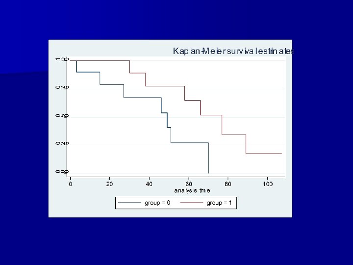
Comparison of survival curve n One important aspect of survival analysis is the comparison of survival curves n Null hypothesis: S 1(t)=S 2(t) n Method: log-rank test

Example Untreated Treated Patient Time 1 30 2 8+ 2 38 3 15 3 52+ 4 27+ 4 58 5 32 5 66 6 46 6 73+ 7 49 7 77 8 51 8 89 9 55+ 9 107+ 10 70

Log-rank test-technical n To compare survival curves, a log-rank test creates 2 x 2 tables at each event time and combines across the tables – Similar to MH-test a c 2 statistic with 1 degree of freedom (for a two sample comparison) and a p-value n Same procedure for hypothesis testing n Provides

Hypothesis test 1) 2) 3) 4) 5) 6) 7) H 0: S 1(t)=S 2(t) Time to event outcome, dichotomous predictor Log rank test Test statistic: c 2=4. 4 p-value=0. 036 Since the p-value is less than 0. 05, we reject the null hypothesis We conclude that there is a significant difference in the survival time in the treated compared to untreated

p-value

Notes n Inspection of Kaplan-Meier curve will allow you to determine which of the groups had the significantly longer survival time n Other tests are possible – Gehan’s generalized Wilcoxon test – Tarone-Ware test – Peto-Prentice test n Generally give similar results, but emphasize different parts of survival curve