Surveying II Lecture 6 Error theory Random error

Surveying II. Lecture 6. Error theory. Random error. The mean error and the weight. Propagation of mean error.

Types of errors There are several types of error that can occur, with different characteristics. Blunders Such as miscounting the number of tape lengths when measuring long distances or transposing numbers when booking. Can occur during the whole surveying process, including observing, booking, computing or plotting. Solution: Creating suitable procedures, and checking the measurements. The effect of a blunder is much larger than the acceptable error of the applied measurement technique. Probability theory

Types of errors Systematic errors arise from sources that act in a similar manner on observations. Examples: • expansion of steel tapes due to temperature changes • frequency changes in electromagnetic distance measurements These errors are dangerous, when we have to add observations, because they act in the same direction. Hence the total effect is the sum of each error. Solution: Calibrating the instruments - comparing the observations with other observations made by other instruments.

Types of errors Random errors All the discrepancies remaining once the blunders and systematic errors have been eliminated. Even when a quantity is measured many times with the same technology and instrumentation, it is highly unlikely that the results would be identical. Although these errors are called random, they have the following charachteristics: • small errors occur more frequently than large ones • positive and negative errors are equally likely • very large errors occur rarely Due to this, the normal statistical distribution can be assumed. Solution: Repetitions of observations.

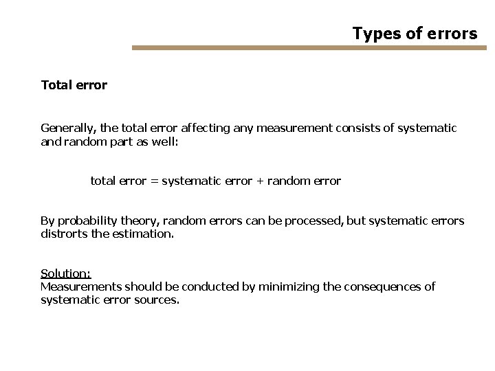
Types of errors Total error Generally, the total error affecting any measurement consists of systematic and random part as well: total error = systematic error + random error By probability theory, random errors can be processed, but systematic errors distrorts the estimation. Solution: Measurements should be conducted by minimizing the consequences of systematic error sources.

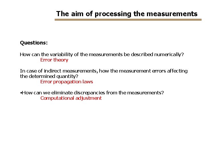
The aim of processing the measurements Questions: How can the variability of the measurements be described numerically? Error theory In case of indirect measurements, how the measurement errors affecting the determined quantity? Error propagation laws • How can we eliminate discrepancies from the measurements? Computational adjustment

Basics of error theory Probabilistic Variables (PV): quantities on which random processes has an effect. Discrete PV: the variable can have a unique number of values. Continuous PV: the variable can have infinite number of values.

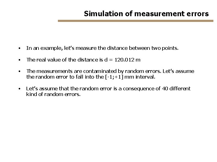
Simulation of measurement errors • In an example, let’s measure the distance between two points. • The real value of the distance is d = 120. 012 m • The measurements are contaminated by random errors. Let’s assume the random error to fall into the [-1; +1] mm interval. • Let’s assume that the random error is a consequence of 40 different kind of random errors.

Simulation of measurement errors We are looking for the answer to the following questions: • What is the integrated error of the different sources on the measured distance? • In case of repeated measurements, how the results of the measurements vary? • Between what bounds fall the results of the measurements?

Simulation of measurement errors Example in the Excel table

Simulation of measurement errors Conclusions The integrated error of different error sources are notably smaller than the product of the number of error sources and the maximal errors. It is the consequence of that the random errors may cancel each other. Most of the measurements are close to the real value. Regardless random errors contaminating the measurements, the mean value of the measurements is very close to the real value.

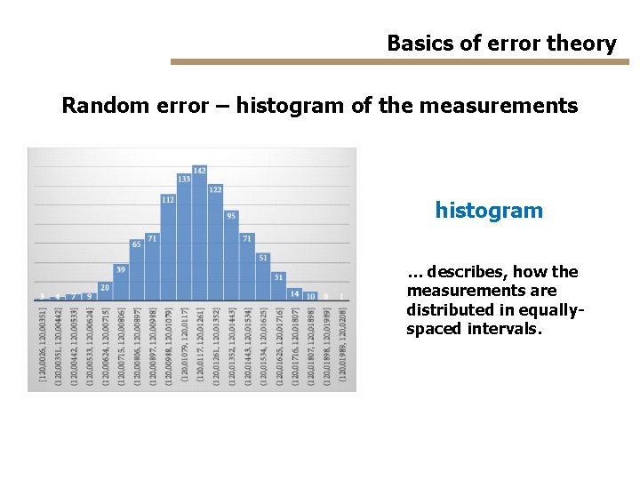
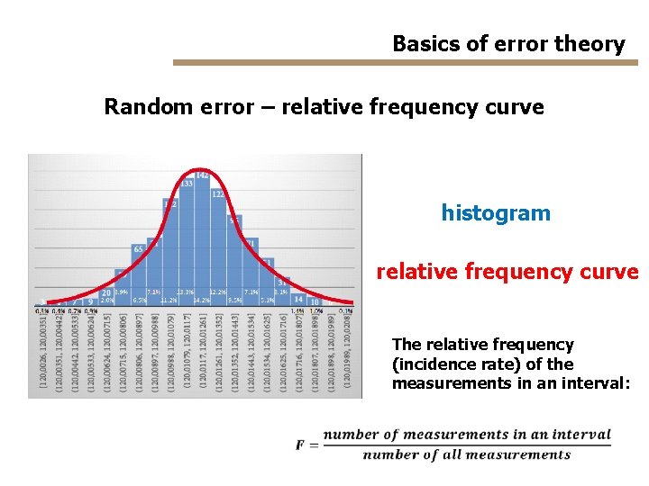
Basics of error theory Random error – histogram of the measurements histogram … describes, how the measurements are distributed in equallyspaced intervals.

Basics of error theory Random error – relative frequency curve histogram relative frequency curve The relative frequency (incidence rate) of the measurements in an interval:

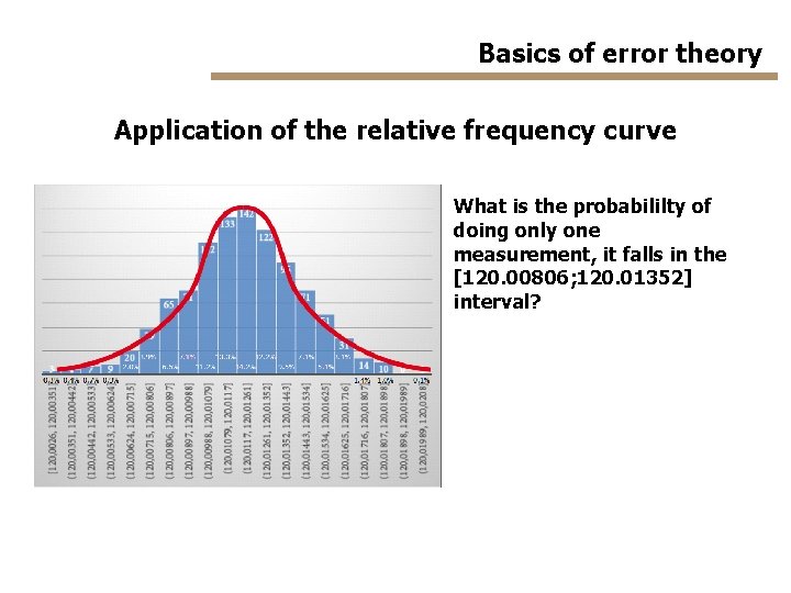
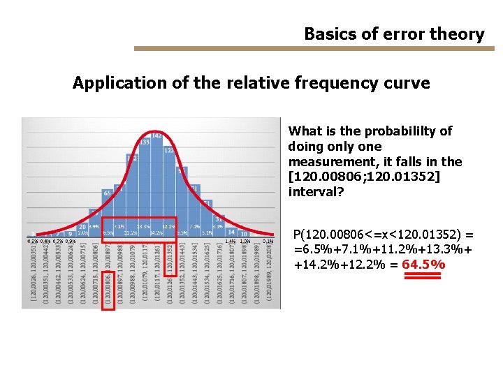
Basics of error theory Application of the relative frequency curve What is the probabililty of doing only one measurement, it falls in the [120. 00806; 120. 01352] interval?

Basics of error theory Application of the relative frequency curve What is the probabililty of doing only one measurement, it falls in the [120. 00806; 120. 01352] interval? P(120. 00806<=x<120. 01352) = =6. 5%+7. 1%+11. 2%+13. 3%+ +14. 2%+12. 2% = 64. 5%

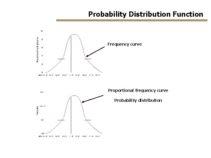
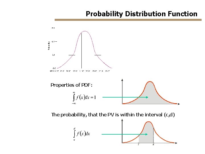
Probability Distribution Function Frequency curve Proportional frequency curve Probability distribution

Probability Distribution Function Properties of PDF: The probability, that the PV is within the interval (c, d)

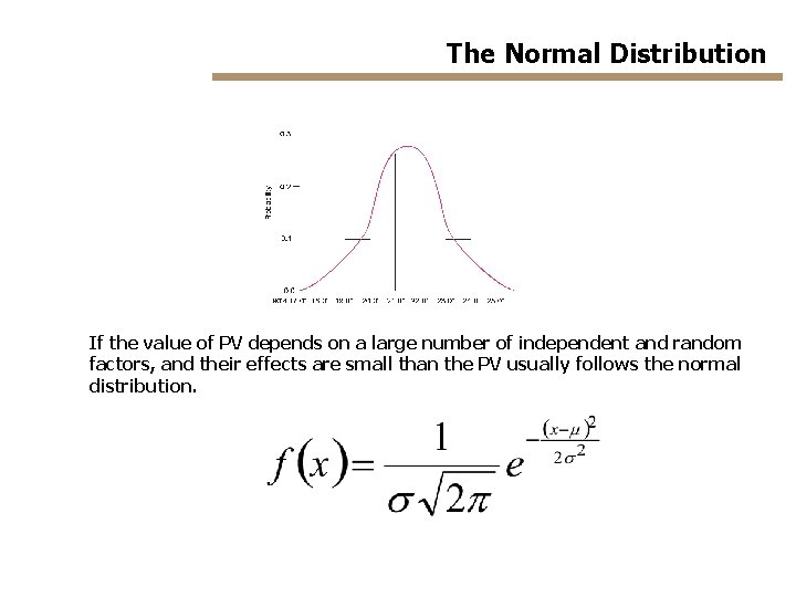
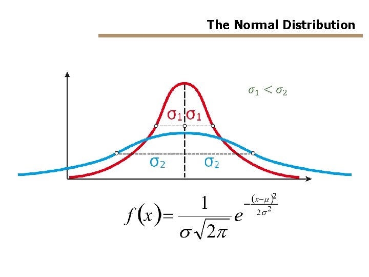
The Normal Distribution If the value of PV depends on a large number of independent and random factors, and their effects are small than the PV usually follows the normal distribution.

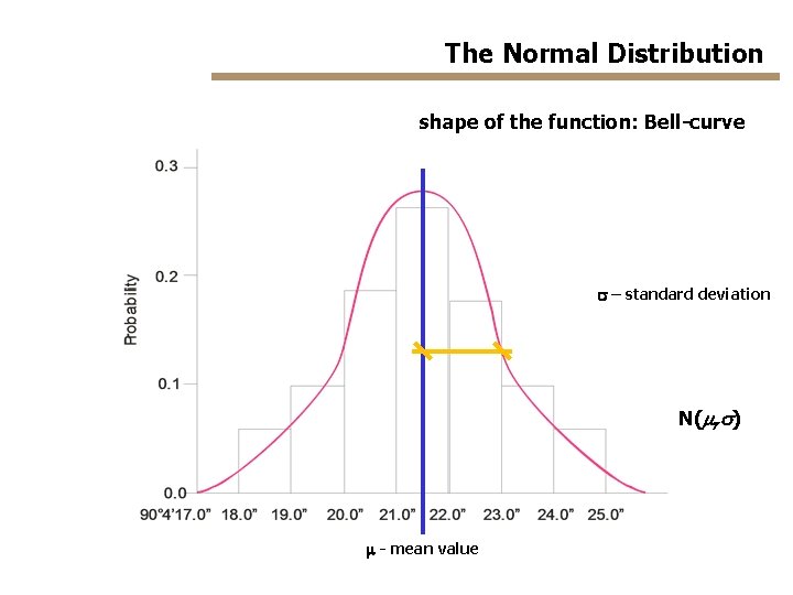
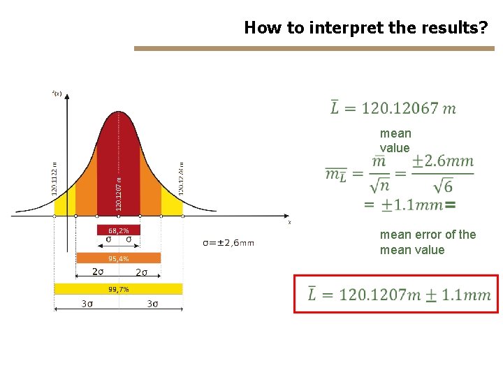
The Normal Distribution shape of the function: Bell-curve s – standard deviation N(m, s) m - mean value

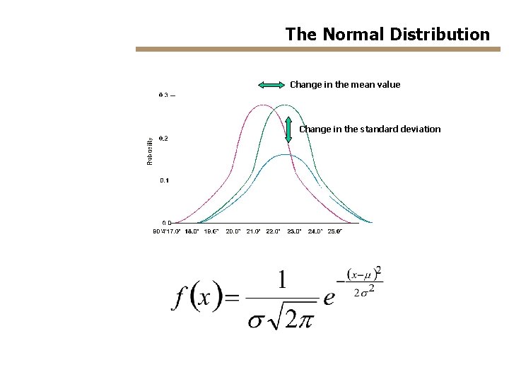
The Normal Distribution Change in the mean value Change in the standard deviation

The Normal Distribution

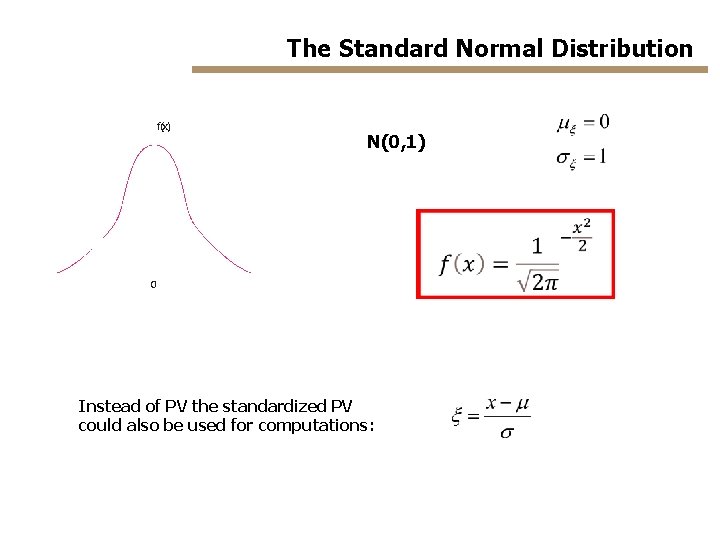
The Standard Normal Distribution N(0, 1) Instead of PV the standardized PV could also be used for computations:

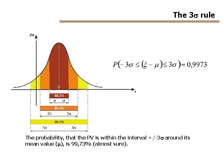
The 3 s rule The probability, that the PV is within the interval +/-3 s around its mean value (m), is 99, 73% (almost sure).

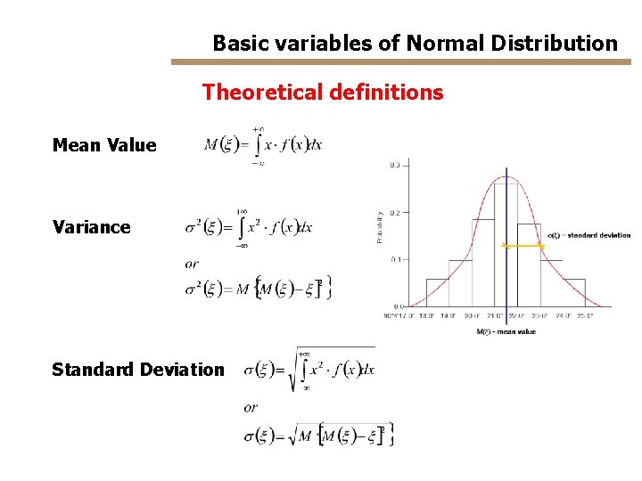
Basic variables of Normal Distribution Theoretical definitions Mean Value Variance Standard Deviation

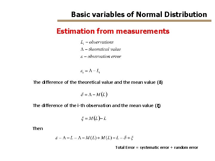
Basic variables of Normal Distribution Estimation from measurements The difference of theoretical value and the mean value (d) The difference of the i-th observation and the mean value (x) Then Total Error = systematic error + random error

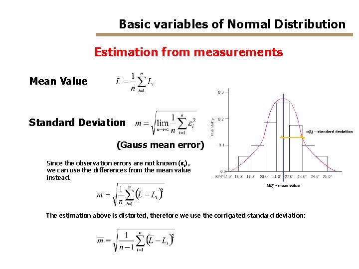
Basic variables of Normal Distribution Estimation from measurements Mean Value Standard Deviation (Gauss mean error) Since the observation errors are not known (ei), we can use the differences from the mean value instead. The estimation above is distorted, therefore we use the corrigated standard deviation:

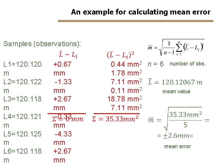
An example for calculating mean error Samples (observations): L 1=120. 120 m L 2=120. 122 m L 3=120. 118 m L 4=120. 121 m L 5=120. 125 m L 6=120. 118 m +0. 67 mm -1. 33 mm +2. 67 mm -0. 33 mm -4. 33 mm +2. 67 mm 0. 44 mm 2 n = 6 number of obs. 1. 78 mm 2 7. 11 mm 2 0. 11 mm 2 mean value 18. 78 mm 2 7. 11 mm 2 mean error

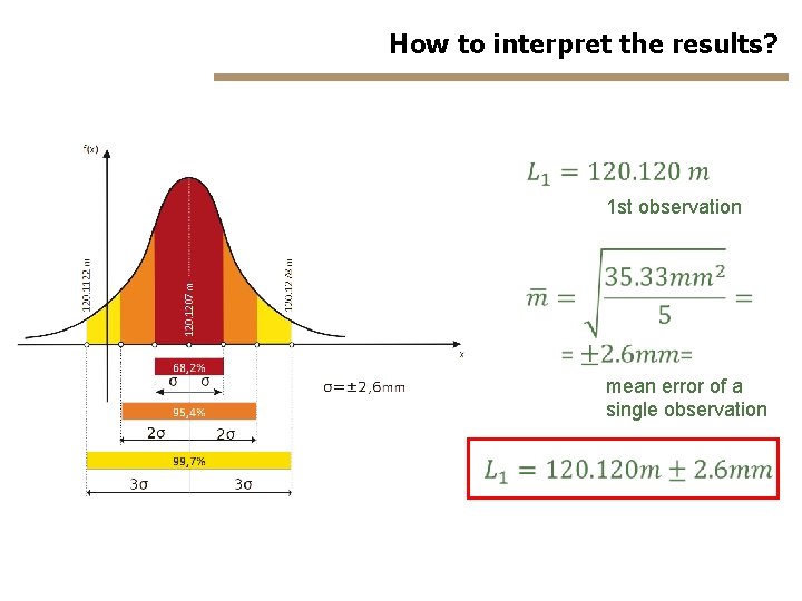
How to interpret the results? 1 st observation mean error of a single observation

How to interpret the results? mean value mean error of the mean value