Survey and Recent Results Robust Geometric Computation Chee

Survey and Recent Results: Robust Geometric Computation Chee Yap Department of Computer Science Courant Institute New York University Oct 18, 2001 Talk @ MIT 1

OVERVIEW n n Part I: Non. Robustness Survey Part II: Exact Geometric Computation F Core Library F Constructive Root Bounds n Part III: New Directions F Moore’s Law and Non. Robustness F Certification Paradigm n Oct 18, 2001 Conclusion Talk @ MIT 2

Numerical Nonrobustnes s Phenomenon Oct 18, 2001 Talk @ MIT 3

Part I: OVERVIEW n n Oct 18, 2001 The Phenomenon What is Geometric? Taxonomy of Approaches EGC and relatives Talk @ MIT 4

Numerical Nonrobustness n Non-robustness phenomenon y crash, n inconsistent state, intermittent Round-off errors y benign vs. catastrophic y quantitative vs. qualitative Oct 18, 2001 Talk @ MIT 5

Examples n Intersection of 2 lines y check n Mesh Generation y point n if intersection point is on line classification error (dirty meshes) Trimmed algebraic patches in CAD y bounding curves are approximated leading to topological inconsistencies n Front Tracking Physics Simulation y front Oct 18, 2001 surface becomes self-intersecting Talk @ MIT 6

Responses to Non-robustness n n n Oct 18, 2001 “It is a rare event” “Use more stable algorithms” “Avoid ill-conditioned inputs” “Epsilon-tweaking” “There is no solution” “Our competitors couldn’t do it, so we don’t have to bother” Talk @ MIT 7

Impact of Nonrobustness n n Acknowledged, seldom demanded Economic/productivity Impact y barrier to full automation y scientist/programmer productivity y mission critical computation fail F n Patriot missile, Ariadne Rocket E. g. Mesh generation ya preliminary step for simulations y 1 failure/5 million cells [Aftosmis] y tweak data if failure Oct 18, 2001 Talk @ MIT 8

What is Special about Geometry? Oct 18, 2001 Talk @ MIT 9

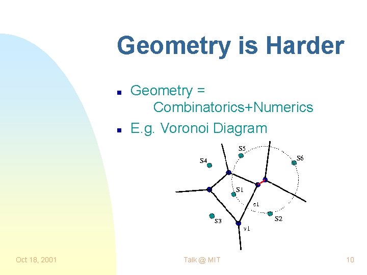
Geometry is Harder n n Oct 18, 2001 Geometry = Combinatorics+Numerics E. g. Voronoi Diagram Talk @ MIT 10

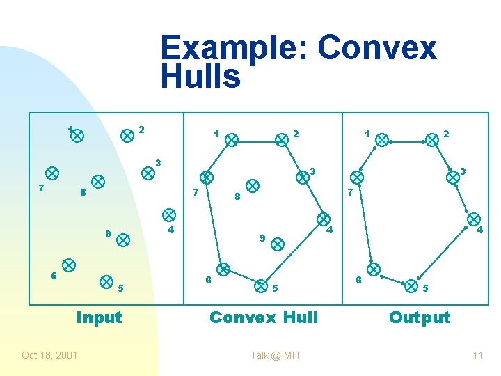
Example: Convex Hulls 1 2 3 7 6 7 Input Oct 18, 2001 3 7 8 4 5 2 3 8 9 1 4 9 6 5 Convex Hull Talk @ MIT 4 6 5 Output 11

Consistency n Geometric Object D = (G, L, P) G=graph, L=labeling of G n Consistency Relation (P) E. g. D is convex hull or Voronoi n diagram Qualitative error inconsistency n Oct 18, 2001 Talk @ MIT 12

Examples/Nonexam ples n Consistency is critical y matrix multiplication y shortest paths in graphs (e. g. Djikstra’s algorithm) y sorting and geometric sorting y Euclidean shortest paths Oct 18, 2001 Talk @ MIT 13

Taxonomy of Approaches Oct 18, 2001 Talk @ MIT 14

Gold Standard n n Must understand the dominant mode of numerical computing “F. P. Mode” : y machine floating point y fixed precision (single/double/quad) y IEEE 754 Standard n What does the IEEE standard do for nonrobustness? Reduces but not eliminate it. Main contribution is cross-platform predictability. n Oct 18, 2001 Historical Note Talk @ MIT 15

Type I Approaches n Basic Philosophy: to make the fast but imprecise (IEEE) arithmetic robust n Taxonomy y arithmetic (FMA, scalar vector, sli, etc) y finite resolution predicates ( -tweaking, - predicates [Guibas-Salesin-Stolfi’ 89]) y finite resolution geometry (e. g. , grids) y topology oriented approach [Sugihara-Iri’ 88] Oct 18, 2001 Talk @ MIT 16

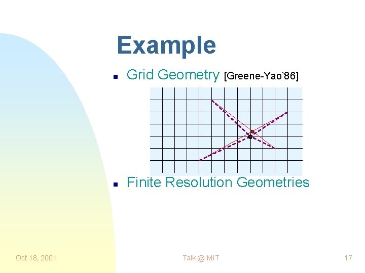
Example Oct 18, 2001 n Grid Geometry [Greene-Yao’ 86] n Finite Resolution Geometries Talk @ MIT 17

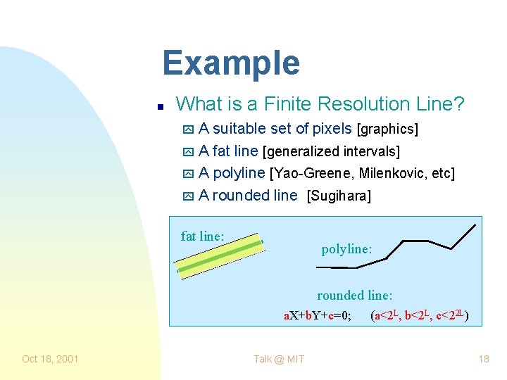
Example n What is a Finite Resolution Line? y. A suitable set of pixels [graphics] y A fat line [generalized intervals] y A polyline [Yao-Greene, Milenkovic, etc] y A rounded line [Sugihara] fat line: polyline: rounded line: a. X+b. Y+c=0; Oct 18, 2001 Talk @ MIT (a<2 L, b<2 L, c<22 L) 18

Example n Topology Oriented Approach of Sugihara-Iri: Voronoi diagram of 1 million points n n n Oct 18, 2001 Priority of topological part over numerical part Identify relevant and maintainable properties: e. g. planarity Issue: which properties to choose? Talk @ MIT 19

Exact Approach n n Idea: avoid all errors Big number packages (big integers, big rationals, big floats, etc) n n Only rational problems are exact Even this is a problem [Yu’ 92, Karasick. Lieber-Nackman’ 89] Oct 18, 2001 Talk @ MIT 20

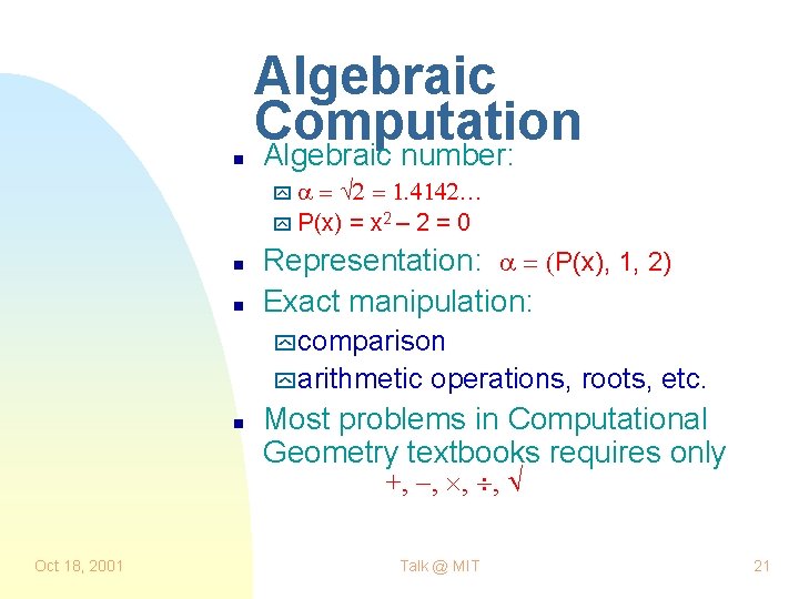
n Algebraic Computation Algebraic number: y y P(x) = x 2 – 2 = 0 n n Representation: P(x), 1, 2) Exact manipulation: y comparison y arithmetic n operations, roots, etc. Most problems in Computational Geometry textbooks requires only +, –, , , Oct 18, 2001 Talk @ MIT 21

Type II Approach n Basic Philosophy: to make slow but error-free computation more efficient n Taxonomy y Exact Arithmetic (naïve approach) y Expression packages y Compiler techniques y Consistency approach y Exact Geometric Computation (EGC) Oct 18, 2001 Talk @ MIT 22

Consistency Approach n n Goal: ensure that no decisions are contradictory Parsimonious Algorithms [Fortune’ 89] : only make tests that are independent of previous results n Oct 18, 2001 NP-hard but in PSPACE Talk @ MIT 23

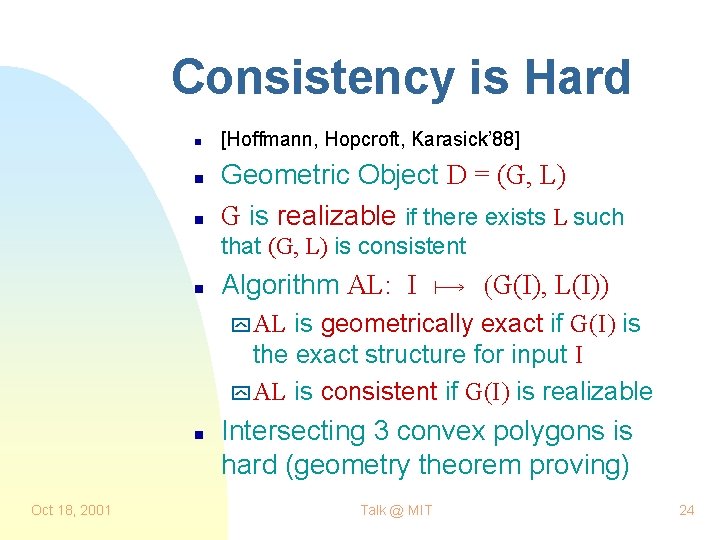
Consistency is Hard n n n [Hoffmann, Hopcroft, Karasick’ 88] Geometric Object D = (G, L) G is realizable if there exists L such that (G, L) is consistent n Algorithm AL: I G(I), L(I)) is geometrically exact if G(I) is the exact structure for input I y AL is consistent if G(I) is realizable y AL n Oct 18, 2001 Intersecting 3 convex polygons is hard (geometry theorem proving) Talk @ MIT 24

Exact Geometric Computation Oct 18, 2001 Talk @ MIT 25

Part II: OVERVIEW n n n Oct 18, 2001 Exact Geometric Computing (EGC) The Core Library Constructive Root Bounds Talk @ MIT 26

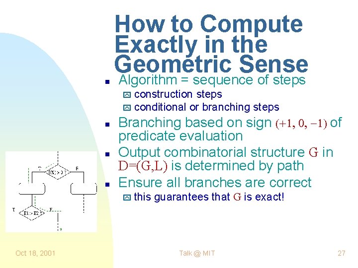
n How to Compute Exactly in the Geometric Sense Algorithm = sequence of steps y construction steps y conditional or branching steps n n n Branching based on sign of predicate evaluation Output combinatorial structure G in D=(G, L) is determined by path Ensure all branches are correct y this Oct 18, 2001 guarantees that G is exact! Talk @ MIT 27

Exact Geometric Computation (EGC) n n Exactness in the Geometry, NOT the arithmetic (cf. geometric exactness) Simple but profound implications y We can now use approximate arithmetic [Dube-Yap’ 94] y EGC tells us exactly how much precision is needed n No unusual geometries y No need to invent new algorithms -“standard” algorithms apply y no unusual geometries n General solution (algebraic case) y Not Oct 18, 2001 algorithm-specific solutions! Talk @ MIT 28

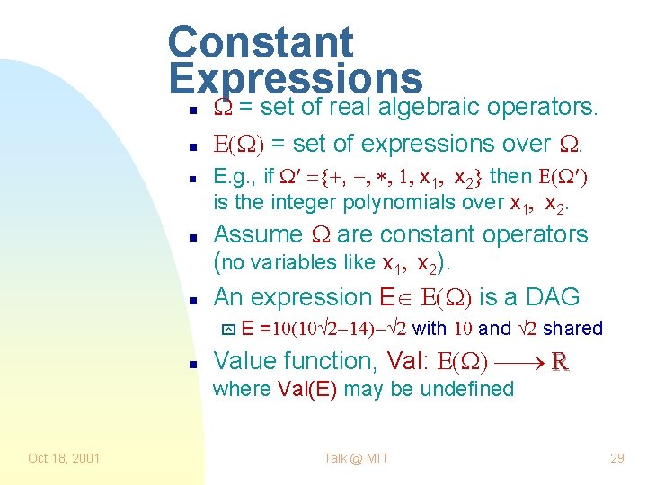
Constant Expressions n n n = set of real algebraic operators. = set of expressions over . E. g. , if , x 1 x 2 then is the integer polynomials over x 1 x 2. Assume are constant operators (no variables like x 1 x 2). An expression E is a DAG y. E n = with and shared Value function, Val: R where Val(E) may be undefined Oct 18, 2001 Talk @ MIT 29

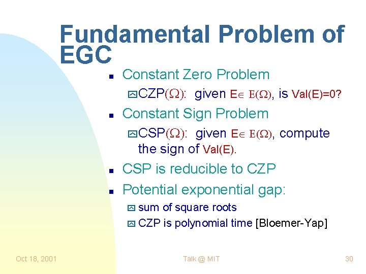
Fundamental Problem of EGC n Constant Zero Problem y CZP : n given E , is Val(E)=0? Constant Sign Problem y CSP : given E , compute the sign of Val(E). n n CSP is reducible to CZP Potential exponential gap: y sum of square roots y CZP is polynomial time [Bloemer-Yap] Oct 18, 2001 Talk @ MIT 30

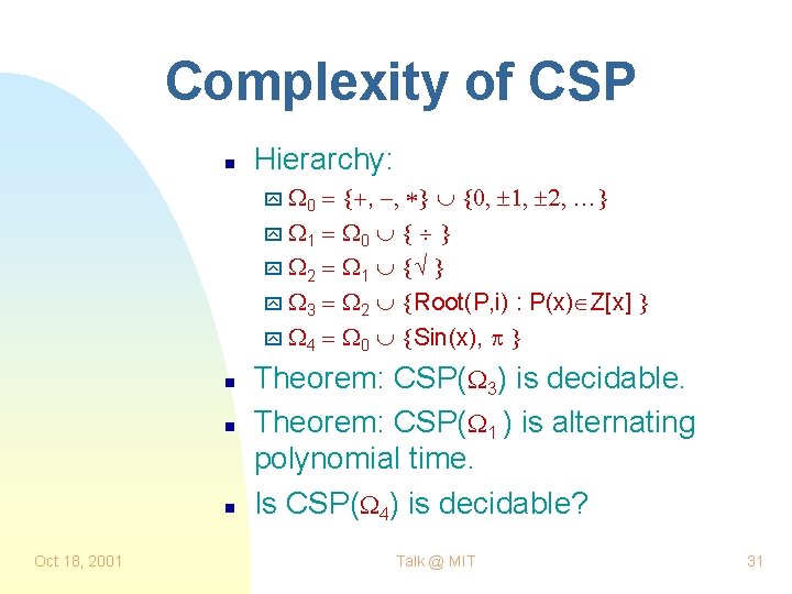
Complexity of CSP n Hierarchy: y 0 , y 1 0 y 2 1 y 3 2 Root(P, i) : P(x) Z[x] y 4 0 Sin(x), n n n Oct 18, 2001 Theorem: CSP( 3) is decidable. Theorem: CSP( 1 ) is alternating polynomial time. Is CSP( 4) is decidable? Talk @ MIT 31

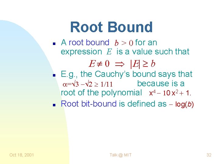
Root Bound n A root bound b > 0 for an expression E is a value such that E ¹ Þ E b n n Oct 18, 2001 E. g. , the Cauchy’s bound says that because is a = root of the polynomial x 4 0 x 2 1. Root bit-bound is defined as log(b) Talk @ MIT 32

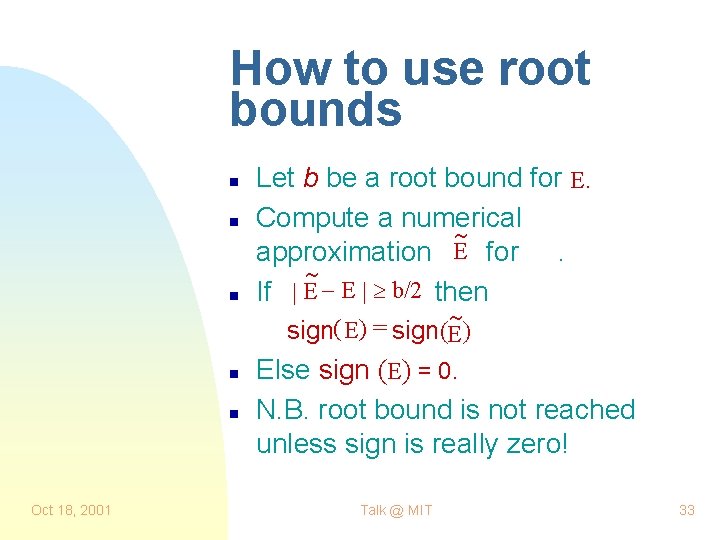
How to use root bounds n n n Let b be a root bound for E. Compute a numerical approximation E for. If E E b/2 then sign( E) = sign(E) n n Oct 18, 2001 Else sign (E) = 0. N. B. root bound is not reached unless sign is really zero! Talk @ MIT 33

Nominally Exact Inputs n n EGC Inputs are exact and consistent Why care about exactness if the input is inexact? Because EGC is the easiest method to ensure consistency. Oct 18, 2001 Talk @ MIT 34

Core Library Oct 18, 2001 Talk @ MIT 35

EGC Libraries n n GOAL: any programmer may routinely construct robust programs* Current Libraries: y Real/Expr [Yap-Dube’ 94] y LEDA real [Burnikel et al’ 99] y Core Library [Karamcheti et al’ 99] Oct 18, 2001 Talk @ MIT 36

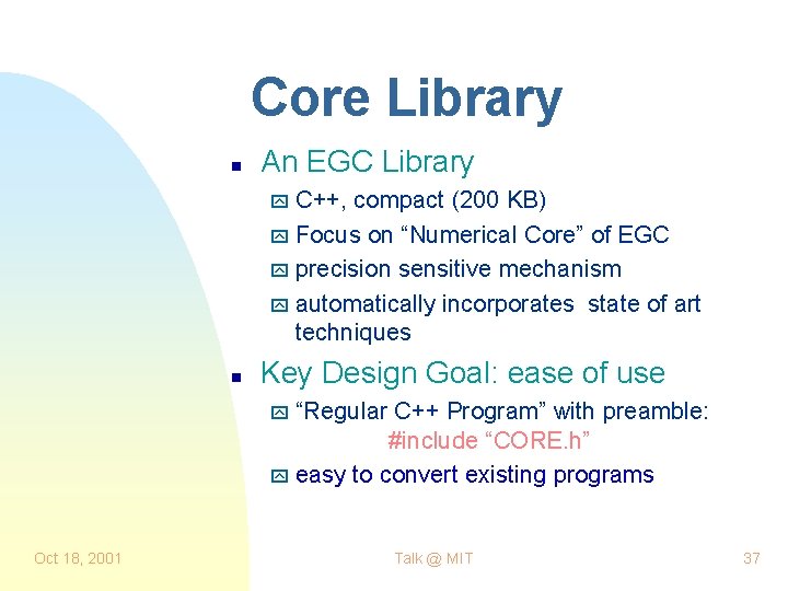
Core Library n An EGC Library y C++, compact (200 KB) y Focus on “Numerical Core” of EGC y precision sensitive mechanism y automatically incorporates state of art techniques n Key Design Goal: ease of use y “Regular C++ Program” with preamble: #include “CORE. h” y easy to convert existing programs Oct 18, 2001 Talk @ MIT 37

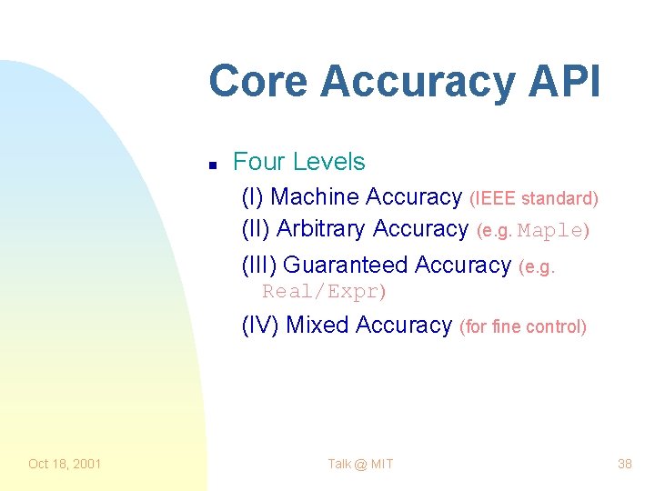
Core Accuracy API n Four Levels (I) Machine Accuracy (IEEE standard) (II) Arbitrary Accuracy (e. g. Maple) (III) Guaranteed Accuracy (e. g. Real/Expr) (IV) Mixed Accuracy (for fine control) Oct 18, 2001 Talk @ MIT 38

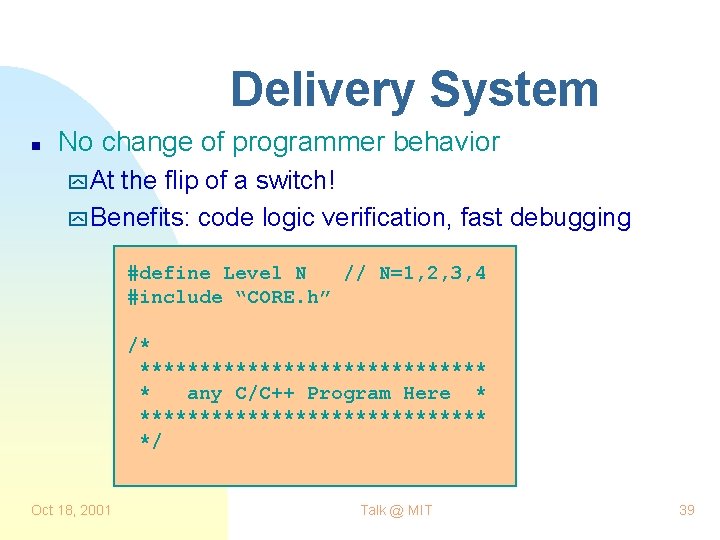
Delivery System n No change of programmer behavior y At the flip of a switch! y Benefits: code logic verification, fast debugging #define Level N // N=1, 2, 3, 4 #include “CORE. h” /* *************** * any C/C++ Program Here * *************** */ Oct 18, 2001 Talk @ MIT 39

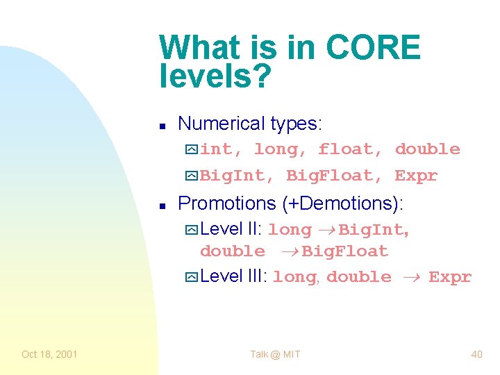
What is in CORE levels? n Numerical types: y int, long, float, double y Big. Int, Big. Float, Expr n Oct 18, 2001 Promotions (+Demotions): y Level II: long Big. Int, double Big. Float y Level III: long, double Expr Talk @ MIT 40

What is in Level III? n n Fundamental gap between Levels II and III Need for iteration: consider a = b + c; n Oct 18, 2001 Precision sensitive evaluation Talk @ MIT 41

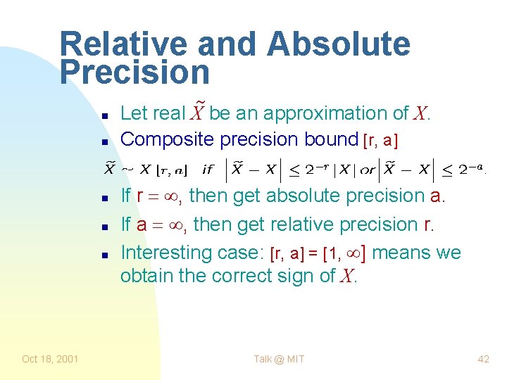
Relative and Absolute Precision n n n Oct 18, 2001 Let real X be an approximation of X. Composite precision bound [r, a] If r , then get absolute precision a. If a , then get relative precision r. Interesting case: [r, a] = [1, ] means we obtain the correct sign of X. Talk @ MIT 42

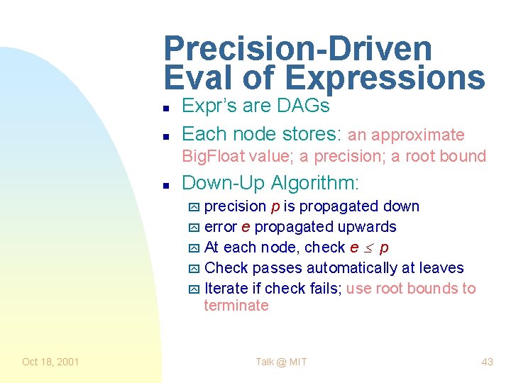
Precision-Driven Eval of Expressions n n Expr’s are DAGs Each node stores: an approximate Big. Float value; a precision; a root bound n Down-Up Algorithm: y precision p is propagated down y error e propagated upwards y At each node, check e p y Check passes automatically at leaves y Iterate if check fails; use root bounds to terminate Oct 18, 2001 Talk @ MIT 43

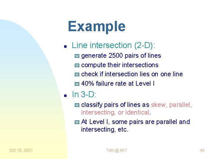
Example n Line intersection (2 -D): y generate 2500 pairs of lines y compute their intersections y check if intersection lies on one line y 40% failure rate at Level I n In 3 -D: y classify pairs of lines as skew, parallel, intersecting, or identical. y At Level I, some pairs are parallel and intersecting, etc. Oct 18, 2001 Talk @ MIT 44

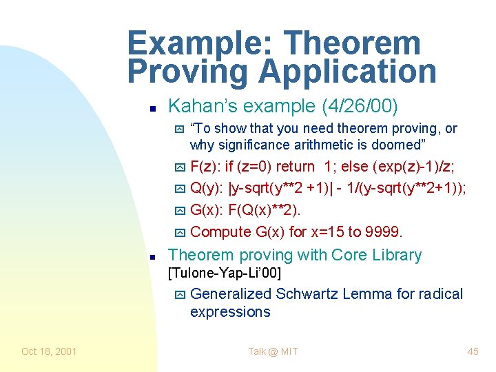
Example: Theorem Proving Application n Kahan’s example (4/26/00) y “To show that you need theorem proving, or why significance arithmetic is doomed” y F(z): if (z=0) return 1; else (exp(z)-1)/z; y Q(y): |y-sqrt(y**2 +1)| - 1/(y-sqrt(y**2+1)); y G(x): F(Q(x)**2). y Compute G(x) for x=15 to 9999. n Theorem proving with Core Library [Tulone-Yap-Li’ 00] y Generalized Schwartz Lemma for radical expressions Oct 18, 2001 Talk @ MIT 45

Constructive Root Bounds Oct 18, 2001 Talk @ MIT 46

Problem of Constructive Root Bounds n n n Oct 18, 2001 Classical root bounds (e. g. Cauchy’s) are not constructive Wanted: recursive rules for a family of expressions to maintain parameters p 1, p 2, etc, for any expression E so that B(p 1, p 2, . . . ) is a root bound for E. We will survey various bounds Talk @ MIT 47

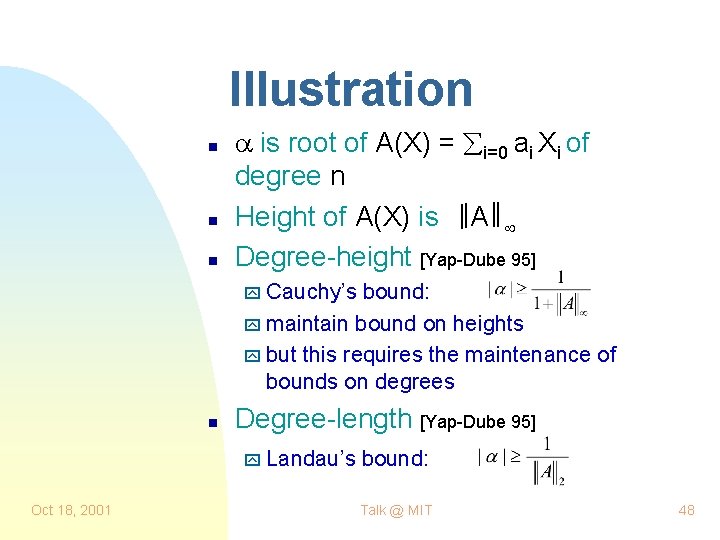
Illustration n is root of A(X) = i=0 ai Xi of degree n Height of A(X) is A Degree-height [Yap-Dube 95] y Cauchy’s bound: y maintain bound on heights y but this requires the maintenance of bounds on degrees n Degree-length [Yap-Dube 95] y Landau’s Oct 18, 2001 bound: Talk @ MIT 48

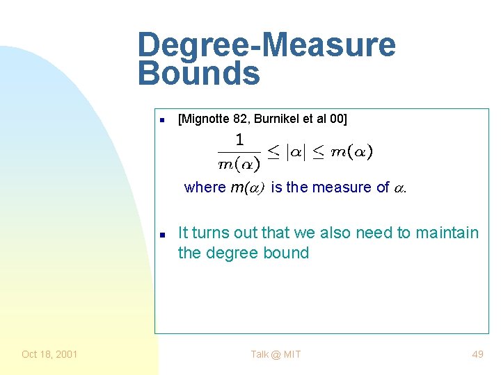
Degree-Measure Bounds n [Mignotte 82, Burnikel et al 00] where m( is the measure of . n Oct 18, 2001 It turns out that we also need to maintain the degree bound Talk @ MIT 49

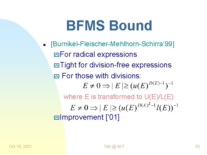
BFMS Bound n [Burnikel-Fleischer-Mehlhorn-Schirra’ 99] y For radical expressions y Tight for division-free expressions y For those with divisions: where E is transformed to U(E)/L(E) y Improvement Oct 18, 2001 [‘ 01] Talk @ MIT 50

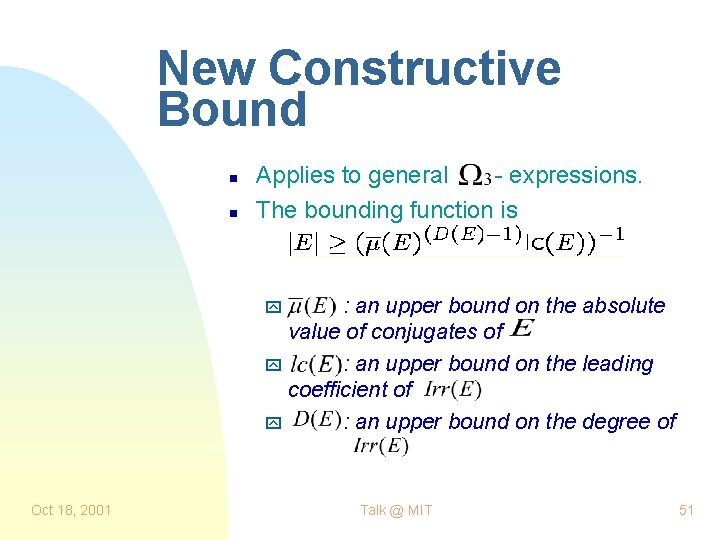
New Constructive Bound n n Applies to general - expressions. The bounding function is : an upper bound on the absolute value of conjugates of y : an upper bound on the leading coefficient of y : an upper bound on the degree of y Oct 18, 2001 Talk @ MIT 51

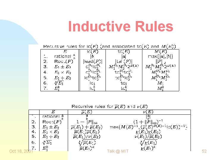
Inductive Rules Oct 18, 2001 Talk @ MIT 52

Comparative Study n n Major open question: is there a root bitbound that depends linearly on degree? No single constructive root bound is always better than the others. y BFMS, degree-measure and our bound y Compare their behavior on interesting classes of expressions: sum of square roots, F continued fraction, etc. F y In Core Library, we compute all three bounds and choose the best one. Oct 18, 2001 Talk @ MIT 53

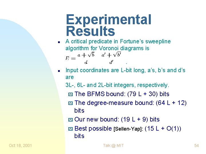
Experimental Results n n A critical predicate in Fortune’s sweepline algorithm for Voronoi diagrams is. Input coordinates are L-bit long, a’s, b’s and d’s are 3 L-, 6 L- and 2 L-bit integers, respectively. y The BFMS bound: (79 L + 30) bits y The degree-measure bound: (64 L + 12) bits y Our new bound: (19 L + 9) bits y Best possible [Sellen-Yap]: (15 L + O(1)) bits Oct 18, 2001 Talk @ MIT 54

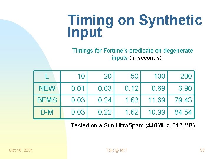
Timing on Synthetic Input Timings for Fortune’s predicate on degenerate inputs (in seconds) L 10 20 50 100 200 NEW 0. 01 0. 03 0. 12 0. 69 3. 90 BFMS 0. 03 0. 24 1. 63 11. 69 79. 43 D-M 0. 03 0. 22 1. 62 10. 99 84. 54 Tested on a Sun Ultra. Sparc (440 MHz, 512 MB) Oct 18, 2001 Talk @ MIT 55

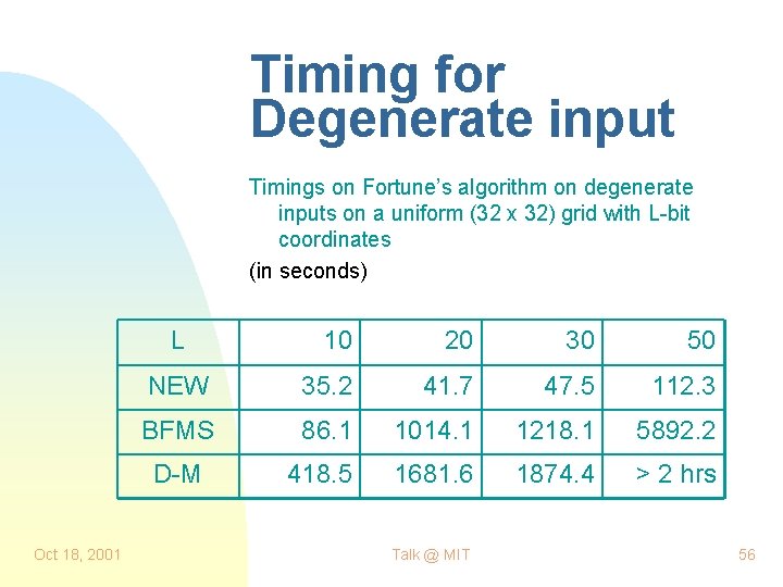
Timing for Degenerate input Timings on Fortune’s algorithm on degenerate inputs on a uniform (32 x 32) grid with L-bit coordinates (in seconds) L Oct 18, 2001 10 20 30 50 NEW 35. 2 41. 7 47. 5 112. 3 BFMS 86. 1 1014. 1 1218. 1 5892. 2 D-M 418. 5 1681. 6 1874. 4 > 2 hrs Talk @ MIT 56

Moore’s Law and Non-robustness Trends Oct 18, 2001 Talk @ MIT 57

Part III: OVERVIEW n n New Directions Robustness as Resource F (or, n Certification Paradigm F (or, Oct 18, 2001 how to exploit Moore’s Law) how to use incorrect algorithms) Talk @ MIT 58

Moore’s Law and Robustness n n Computers are becoming faster (Moore’s Law, 1965) Software becoming less robust y crashes more often y must solves larger/harder problems (e. g. Meshes, CAD) y expectation is increasing n Inverse correlation y is Oct 18, 2001 this inevitable? Talk @ MIT 59

Reversing the Trend n n Robustness: all-or-nothing ? Computational Paradigm y robustness as computational resource y exchange some speed for robustness n Oct 18, 2001 Goal: a positive correlation between Moore’s Law and robustness Talk @ MIT 60

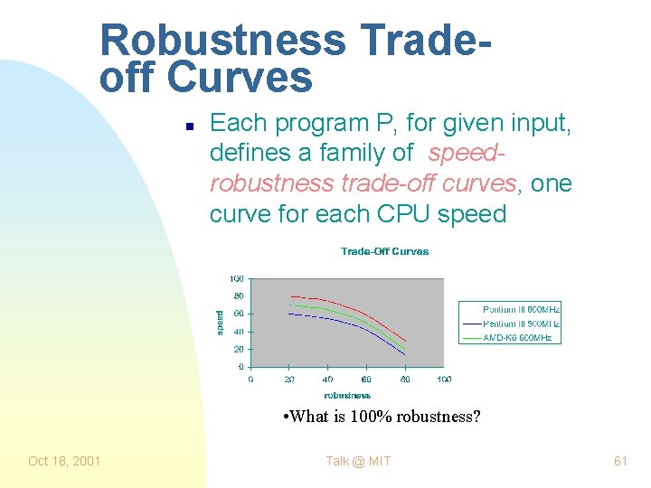
Robustness Tradeoff Curves n Each program P, for given input, defines a family of speedrobustness trade-off curves, one curve for each CPU speed • What is 100% robustness? Oct 18, 2001 Talk @ MIT 61

Computing on the Curve n n Oct 18, 2001 P only needs to be recompiled to operate at any chosen point on a curve. With each new hardware upgrade, we can automatically recompile program to achieve the “sweetspot” on the new curve Talk @ MIT 62

Architecture n Automatically generated Makefiles ya registry of programs that wants to join y sample inputs (various sizes) for each program y robustness targets/parameters y optimization function (e. g. , min acceptable speed) Oct 18, 2001 Talk @ MIT 63

Hardware Change/Upgrade n For given hardware configuration, for each program: y compile different robust versions of the program y run each on the test inputs to determine trade-off curve y optimize the parameters n n n Layer above the usual compiler Application: libraries, CPU upgrades Can be automatic and transparent (like the effects of Moore’s law) Oct 18, 2001 Talk @ MIT 64

Certification Paradigm Oct 18, 2001 Talk @ MIT 65

Another Paradigm Shift n Motivation: programs based on machine arithmetic are fast, but not always correct. n n Oct 18, 2001 Floating point filter phenomenon Need new framework for working with ``useful but incorrect algorithms’’ Talk @ MIT 66

Verification vs. Checking n Program verification movement n (1970 s) Another reason why it failed: y Algorithm: “always correct” y H-algorithm: “always fast, often correct” n Checking paradigm [Blum, Kannan] y use H-algorithms y only check specific input/output pairs, not programs. Oct 18, 2001 Talk @ MIT 67

Checking vs. Certifying n Checker: given an input-output pair, always accept or reject correctly n Certifier (or Filter): given an inputoutput pair, either accept or “unsure” n Why certify? y Certifiers are easier to design y Nontrivial checkers may not be known (e. g. sign of determinant) Oct 18, 2001 Talk @ MIT 68

Filtered Algorithms n How to use Certifiers? Ingredients: Algorithm A F H-algorithm H F Filter or Certifier F F n Basic Architecture y run Oct 18, 2001 H, filter with F, run A if necessary Talk @ MIT 69

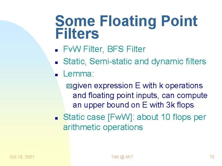
Some Floating Point Filters n n n Fv. W Filter, BFS Filter Static, Semi-static and dynamic filters Lemma: y given expression E with k operations and floating point inputs, can compute an upper bound on E with 3 k flops n Oct 18, 2001 Static case [Fw. W]: about 10 flops per arithmetic operations Talk @ MIT 70

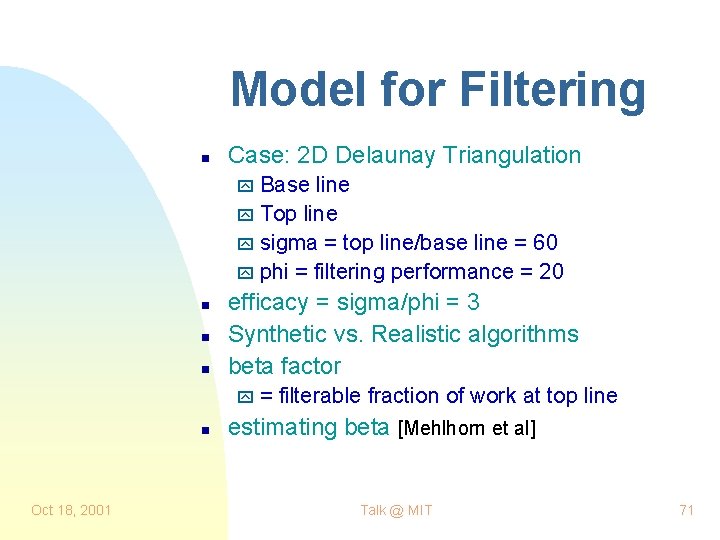
Model for Filtering n Case: 2 D Delaunay Triangulation y Base line y Top line y sigma = top line/base line = 60 y phi = filtering performance = 20 n n n efficacy = sigma/phi = 3 Synthetic vs. Realistic algorithms beta factor y= n Oct 18, 2001 filterable fraction of work at top line estimating beta [Mehlhorn et al] Talk @ MIT 71

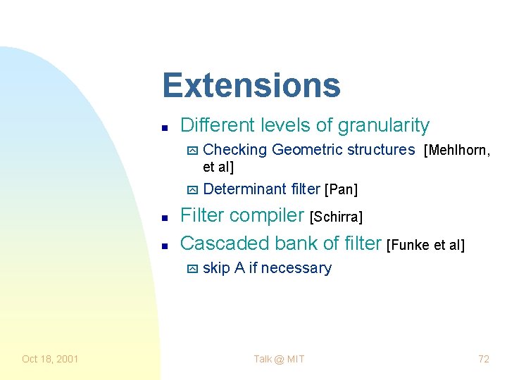
Extensions n Different levels of granularity y Checking Geometric structures [Mehlhorn, et al] y Determinant n n Filter compiler [Schirra] Cascaded bank of filter [Funke et al] y skip Oct 18, 2001 filter [Pan] A if necessary Talk @ MIT 72

Conclusion Oct 18, 2001 Talk @ MIT 73

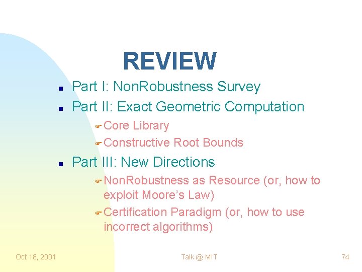
REVIEW n n Part I: Non. Robustness Survey Part II: Exact Geometric Computation F Core Library F Constructive Root Bounds n Part III: New Directions F Non. Robustness as Resource (or, how to exploit Moore’s Law) F Certification Paradigm (or, how to use incorrect algorithms) Oct 18, 2001 Talk @ MIT 74

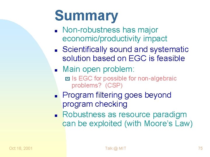
Summary n n n Non-robustness has major economic/productivity impact Scientifically sound and systematic solution based on EGC is feasible Main open problem: y Is EGC for possible for non-algebraic problems? (CSP) n n Oct 18, 2001 Program filtering goes beyond program checking Robustness as resource paradigm can be exploited (with Moore’s Law) Talk @ MIT 75

Download Software n n n Core Library Version 1. 4 small and easy-to-use Project Homepage: http: //cs. nyu. edu/exact/ Oct 18, 2001 Talk @ MIT 76

Last Slide Oct 18, 2001 Talk @ MIT 77

Extras Oct 18, 2001 Talk @ MIT 78

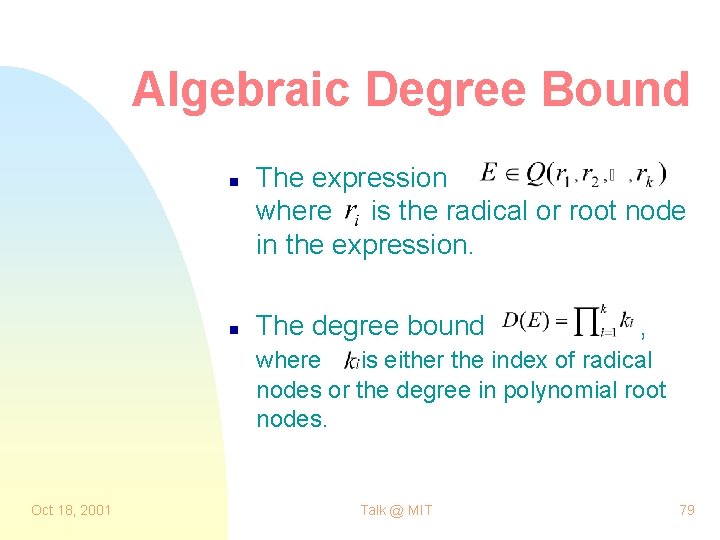
Algebraic Degree Bound n n The expression where is the radical or root node in the expression. The degree bound , where is either the index of radical nodes or the degree in polynomial root nodes. Oct 18, 2001 Talk @ MIT 79

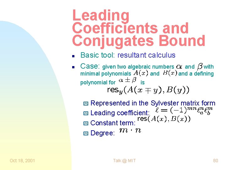
Leading Coefficients and Conjugates Bound n n Basic tool: resultant calculus Case: given two algebraic numbers minimal polynomials polynomial for and with and a defining is y Represented in the Sylvester matrix form y Leading coefficient: y Constant term: y Degree: Oct 18, 2001 Talk @ MIT 80

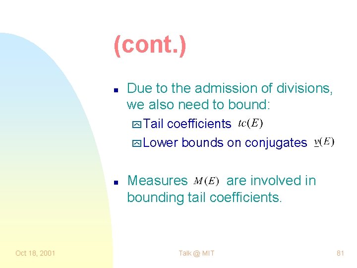
(cont. ) n Due to the admission of divisions, we also need to bound: y Tail coefficients y Lower bounds on conjugates n Oct 18, 2001 Measures are involved in bounding tail coefficients. Talk @ MIT 81

End of Extra Slides Oct 18, 2001 Talk @ MIT 82