Surfaces and Curves Introduction Graphics scenes can contain

Surfaces and Curves

Introduction • Graphics scenes can contain many different kinds of • • objects • No one method can describe all these objects • Accurate models produce realistic displays of scenes • Polygon and quadric surfaces • Spline surfaces and construction techniques • Procedural methods • Physically-based modeling methods • Octree encodings Boundary representations (B-reps) Space-partitioning representations Madhulika (18010), Assistant Professor, LPU.

Polygon Surfaces • The most commonly used boundary represent-ation • All surfaces are described with linear equations • Simplify and speed up surface rendering and display of • • objects Precisely define a polyhedron For non-polyhedron objects, surfaces are tesselated • Commonly used in design and solid modeling • The wireframe outline can be display quickly Madhulika (18010), Assistant Professor, LPU.

Polygon Tables • Specify a polygon surface • Geometric tables • Vertex coordinates • Spatial orientation of the polygon • Attribute tables • Degree of transparency • Surface reflectivity • Texture Madhulika (18010), Assistant Professor, LPU.

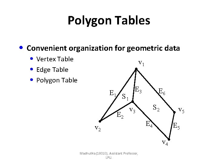
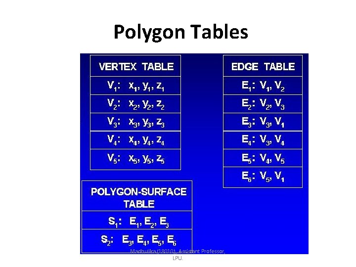
Polygon Tables • Convenient organization for geometric data • Vertex Table • Edge Table • Polygon Table v 1 E 1 S E 3 1 E 2 E 6 S 2 v 3 v 2 v 5 E 4 E 5 v 4 Madhulika (18010), Assistant Professor, LPU.

Polygon Tables Madhulika (18010), Assistant Professor, LPU.

Polygon Tables • Alternative arrangements • Use just two tables: a vertex table and a polygon table • Some edges could get drawn twice • Use only a polygon table • This duplicates coordinate information • Extra information to the data tables • Expand the edge table to include forward pointers into the polygon table • Common edges between polygons • Expand vertex table to contain cross-reference to corresponding edges Madhulika (18010), Assistant Professor, LPU.

Polygon Tables • Additional geometric information • The slope for each edge • Coordinate extents for each polygon • Tests for consistency and completeness • Every vertex is an endpoint for at least two edges • Every edge is part of at least one polygon • Every polygon is closed • Each polygon has at least one shared edge • Every edge referenced by a polygon pointer has a reciprocal pointer back to the polygon Madhulika (18010), Assistant Professor, LPU.

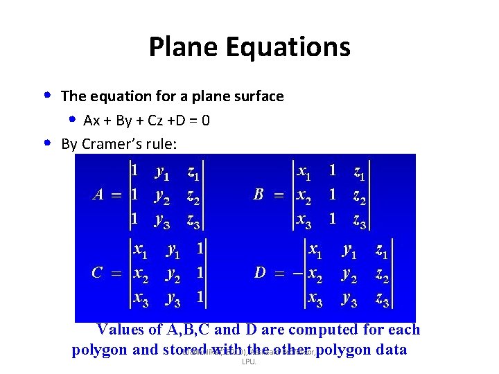
Plane Equations • The equation for a plane surface • Ax + By + Cz +D = 0 • By Cramer’s rule: Values of A, B, C and D are computed for each polygon and stored with the other polygon data Madhulika (18010), Assistant Professor, LPU.

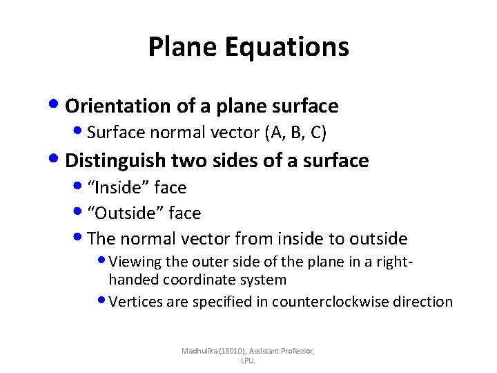
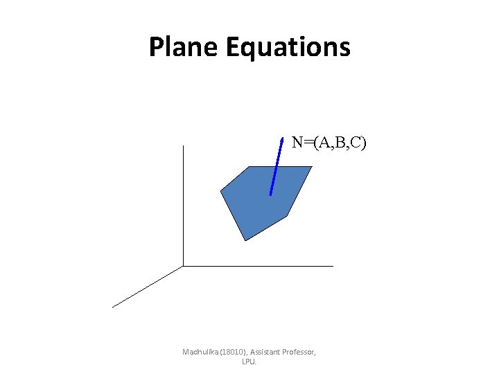
Plane Equations • Orientation of a plane surface • Surface normal vector (A, B, C) • Distinguish two sides of a surface • “Inside” face • “Outside” face • The normal vector from inside to outside • Viewing the outer side of the plane in a right- handed coordinate system • Vertices are specified in counterclockwise direction Madhulika (18010), Assistant Professor, LPU.

Plane Equations N=(A, B, C) Madhulika (18010), Assistant Professor, LPU.

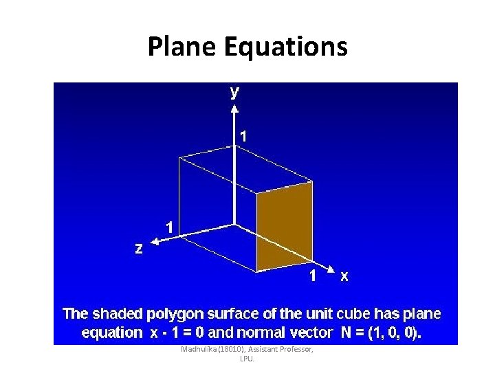
Plane Equations Madhulika (18010), Assistant Professor, LPU.

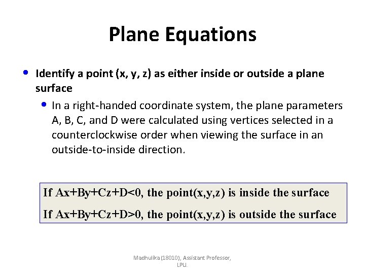
Plane Equations • Identify a point (x, y, z) as either inside or outside a plane surface • In a right-handed coordinate system, the plane parameters A, B, C, and D were calculated using vertices selected in a counterclockwise order when viewing the surface in an outside-to-inside direction. If Ax+By+Cz+D<0, the point(x, y, z) is inside the surface If Ax+By+Cz+D>0, the point(x, y, z) is outside the surface Madhulika (18010), Assistant Professor, LPU.

Curves • Although used for display, bit maps are not appropriate for most computational tasks, which need a three-dimensional representation of the objects composing the image. • Represented skeletally as a wire-frame image, the Utah Teapot is composed of many small polygons. However, even with hundreds of polygons, the image is not smooth. • Smoother representations can be provided by Bezier curves, which have the further advantage of requiring less computer memory. Madhulika (18010), Assistant Professor, LPU.

• Bezier curves are described by cubic equations; a cubic curve is determined by four points or, equivalently, by two points and the curve’s slopes at those points. • Two cubic curves can be smoothly joined by giving them the same slope at the junction. • Bezier curves, and related curves known as Bsplines, were introduced in computer-aided design programs for the modeling of automobile bodies. Madhulika (18010), Assistant Professor, LPU.

Spline • To produce a smooth curve through a designed set of points, a flexible strip called spline is used. • Such a spline curve can be mathematically described with a piecewise cubic polynomial function. Madhulika (18010), Assistant Professor, LPU.

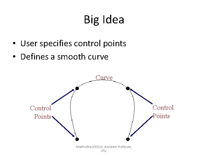
Big Idea • User specifies control points • Defines a smooth curve Control Points Madhulika (18010), Assistant Professor, LPU.

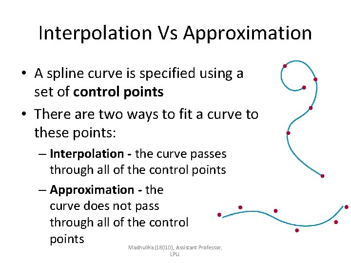
Interpolation Vs Approximation • A spline curve is specified using a set of control points • There are two ways to fit a curve to these points: – Interpolation - the curve passes through all of the control points – Approximation - the curve does not pass through all of the control points Madhulika (18010), Assistant Professor, LPU.

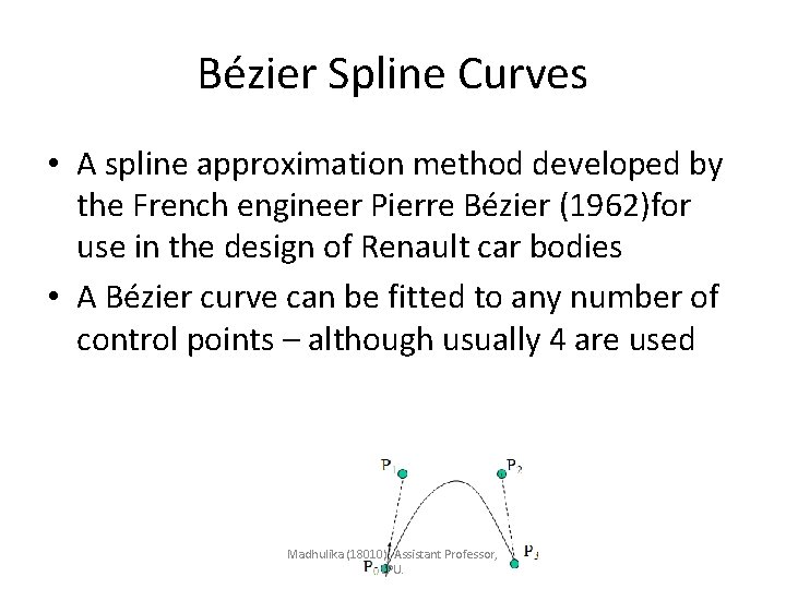
Bézier Spline Curves • A spline approximation method developed by the French engineer Pierre Bézier (1962)for use in the design of Renault car bodies • A Bézier curve can be fitted to any number of control points – although usually 4 are used Madhulika (18010), Assistant Professor, LPU.

• Bezier splines : useful and convenient for curve and surface design • A Bezier curve is a parametric curve frequently used in computer graphics and related fields. • Generalizations of Bezier curves to higher dimensions are called Bezier surfaces, of which the Bezier triangle is a special case. • Bezier curves are used to model smooth curves that can be scaled indefinitely. Madhulika (18010), Assistant Professor, LPU.

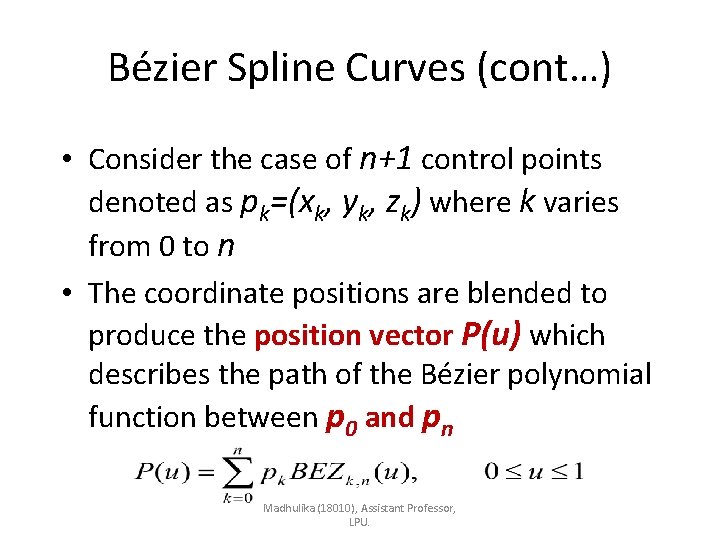
Bézier Spline Curves (cont…) • Consider the case of n+1 control points denoted as pk=(xk, yk, zk) where k varies from 0 to n • The coordinate positions are blended to produce the position vector P(u) which describes the path of the Bézier polynomial function between p 0 and pn Madhulika (18010), Assistant Professor, LPU.

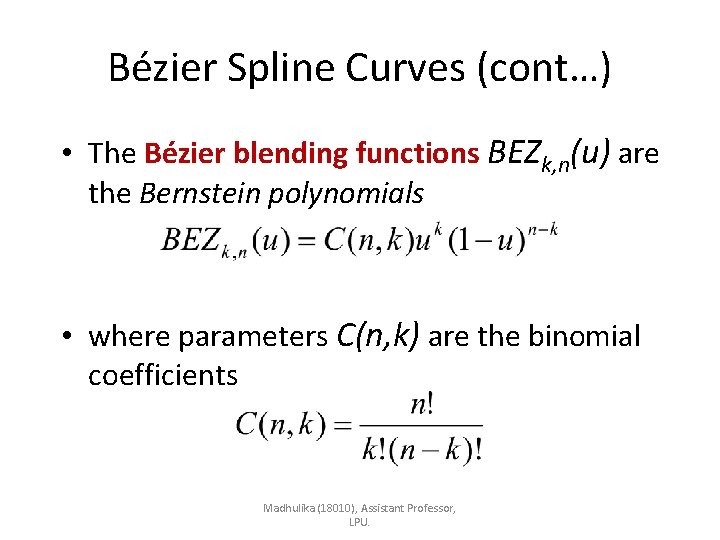
Bézier Spline Curves (cont…) • The Bézier blending functions BEZk, n(u) are the Bernstein polynomials • where parameters C(n, k) are the binomial coefficients Madhulika (18010), Assistant Professor, LPU.

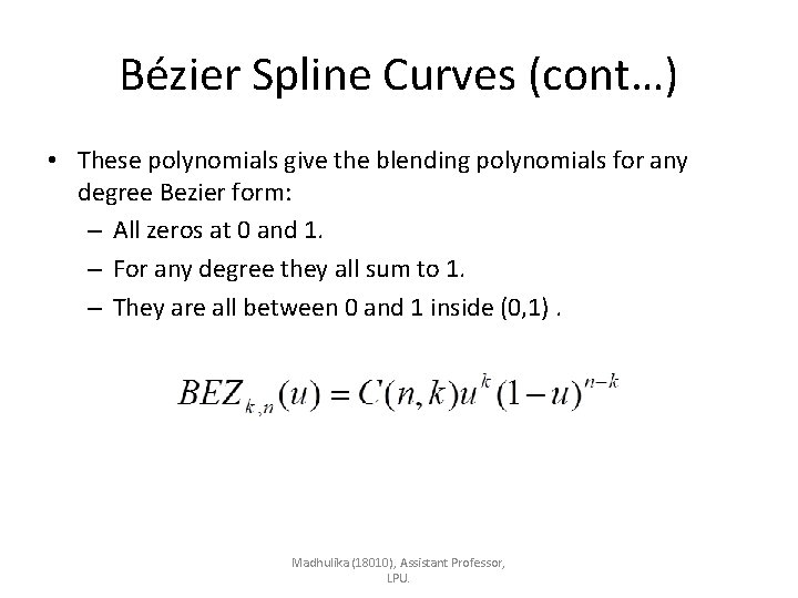
Bézier Spline Curves (cont…) • These polynomials give the blending polynomials for any degree Bezier form: – All zeros at 0 and 1. – For any degree they all sum to 1. – They are all between 0 and 1 inside (0, 1). Madhulika (18010), Assistant Professor, LPU.

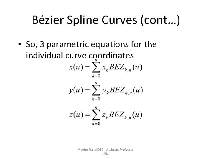
Bézier Spline Curves (cont…) • So, 3 parametric equations for the individual curve coordinates Madhulika (18010), Assistant Professor, LPU.

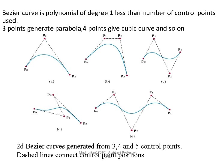
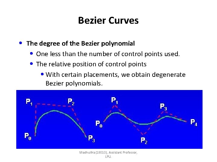
Bezier curve is polynomial of degree 1 less than number of control points used. 3 points generate parabola, 4 points give cubic curve and so on 2 d Bezier curves generated from 3, 4 and 5 control points. Dashed lines connect Madhulika (18010), Assistant Professor, control point positions LPU.

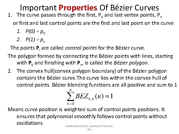
Important Properties Of Bézier Curves 1. The curve passes through the first, P 0 and last vertex points, Pn or first and last control points are the first and last point on the curve 1. P(0) = p 0 2. P(1) = pn The points Pi are called control points for the Bézier curve. The polygon formed by connecting the Bézier points with lines, starting with P 0 and finishing with Pn, is called the Bézier polygon. 2. The convex hull(convex polygon boundary) of the Bézier polygon contains the Bézier curve. The curve lies within the convex hull of control points. Bézier blending functions are all positive and sum to 1 Means curve position is weighted sum of control points positions. It ensures that polynomial smoothly follows control points without oscillations. Madhulika (18010), Assistant Professor, LPU.

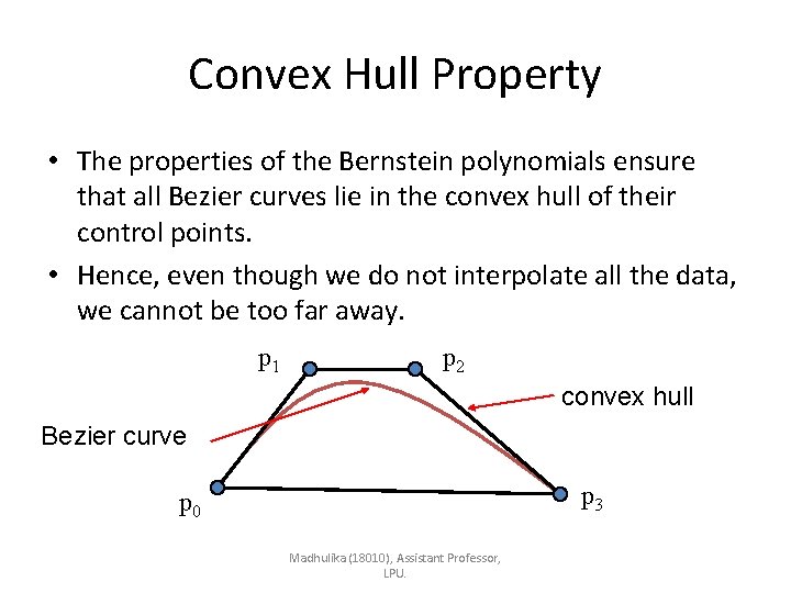
Convex Hull Property • The properties of the Bernstein polynomials ensure that all Bezier curves lie in the convex hull of their control points. • Hence, even though we do not interpolate all the data, we cannot be too far away. p 1 p 2 convex hull Bezier curve p 3 p 0 Madhulika (18010), Assistant Professor, LPU.

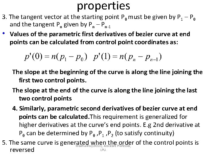
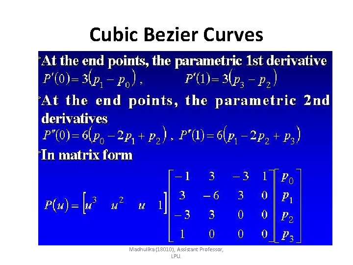
properties 3. The tangent vector at the starting point P 0 must be given by P 1 – P 0 and the tangent Pn given by Pn – Pn-1 • Values of the parametric first derivatives of bezier curve at end points can be calculated from control point coordinates as: The slope at the beginning of the curve is along the line joining the first two control points. The slope at the end of the curve is along the line joining the last two control points 4. Similarly, parametric second derivatives of bezier curve at end points can be calculated. This requirement is generalized for higher derivatives at the curve’s end points. E. g 2 nd derivative at P 0 can be determined by P 0 , P 1 , P 2 (to satisfy continuity) 5. The same curve is generated when the order of the control points is Madhulika (18010), Assistant Professor, LPU. reversed

Bezier Curves • The degree of the Bezier polynomial • One less than the number of control points used. • The relative position of control points • With certain placements, we obtain degenerate Bezier polynomials. Madhulika (18010), Assistant Professor, LPU.

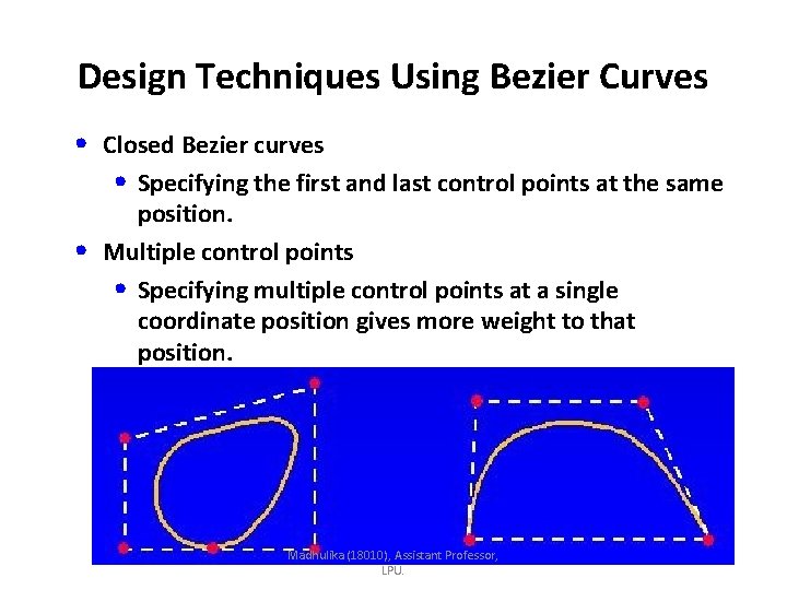
Design Techniques Using Bezier Curves • Closed Bezier curves • Specifying the first and last control points at the same • position. Multiple control points • Specifying multiple control points at a single coordinate position gives more weight to that position. Madhulika (18010), Assistant Professor, LPU.

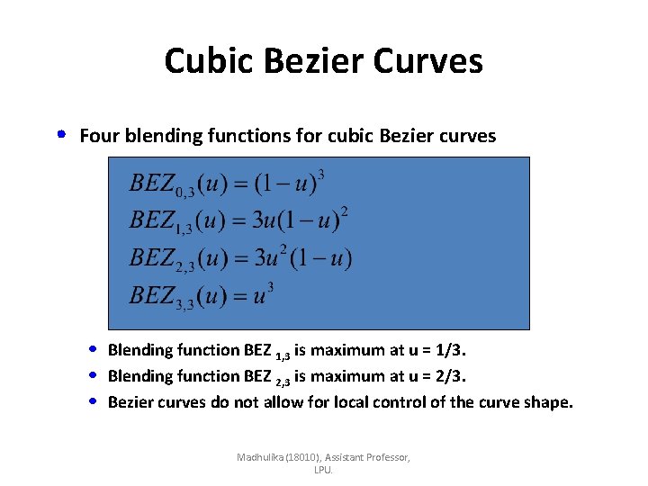
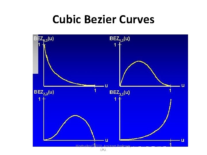
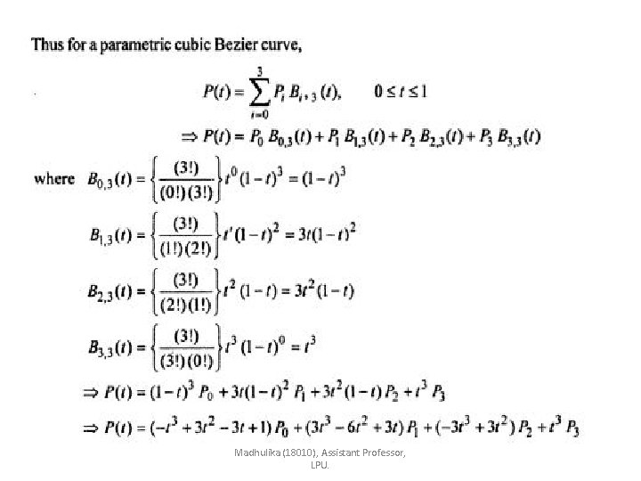
Cubic Bezier Curves • Four blending functions for cubic Bezier curves • Blending function BEZ 1, 3 is maximum at u = 1/3. • Blending function BEZ 2, 3 is maximum at u = 2/3. • Bezier curves do not allow for local control of the curve shape. Madhulika (18010), Assistant Professor, LPU.

Cubic Bezier Curves Madhulika (18010), Assistant Professor, LPU.

Madhulika (18010), Assistant Professor, LPU.

Cubic Bezier Curves Madhulika (18010), Assistant Professor, LPU.

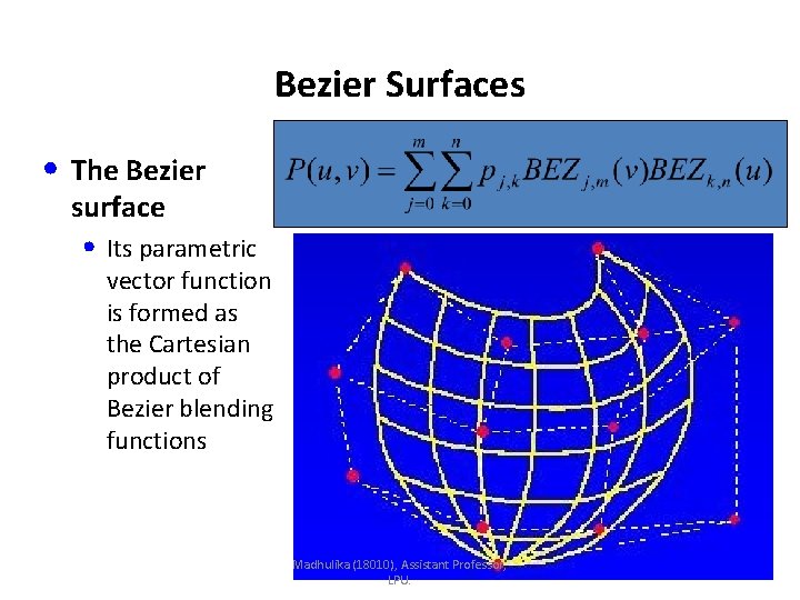
Bezier Surfaces • The Bezier surface • Its parametric vector function is formed as the Cartesian product of Bezier blending functions Madhulika (18010), Assistant Professor, LPU.

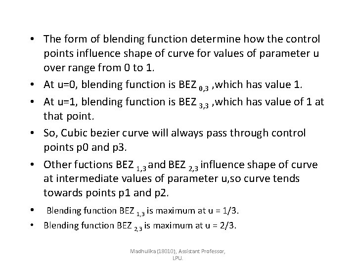
• The form of blending function determine how the control points influence shape of curve for values of parameter u over range from 0 to 1. • At u=0, blending function is BEZ 0, 3 , which has value 1. • At u=1, blending function is BEZ 3, 3 , which has value of 1 at that point. • So, Cubic bezier curve will always pass through control points p 0 and p 3. • Other fuctions BEZ 1, 3 and BEZ 2, 3 influence shape of curve at intermediate values of parameter u, so curve tends towards points p 1 and p 2. • Blending function BEZ 1, 3 is maximum at u = 1/3. • Blending function BEZ 2, 3 is maximum at u = 2/3. Madhulika (18010), Assistant Professor, LPU.

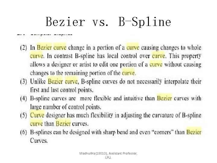
Disadvantages • The degree of the Bezier curve depends on the number of control points. • The Bezier curve lacks local control. Changing the position of one control point affects the entire curve. Madhulika (18010), Assistant Professor, LPU.

Summary • Today we had a look at spline curves and in particular Bézier curves • The whole point is that the spline functions give us an approximation to a smooth curve Madhulika (18010), Assistant Professor, LPU.

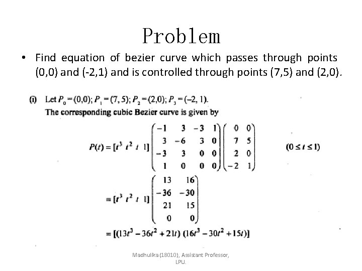
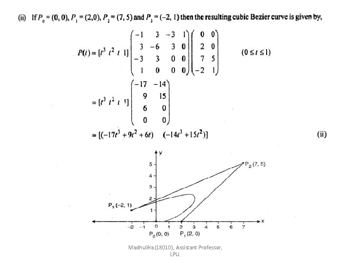
Problem • Find equation of bezier curve which passes through points (0, 0) and (-2, 1) and is controlled through points (7, 5) and (2, 0). Madhulika (18010), Assistant Professor, LPU.

Madhulika (18010), Assistant Professor, LPU.

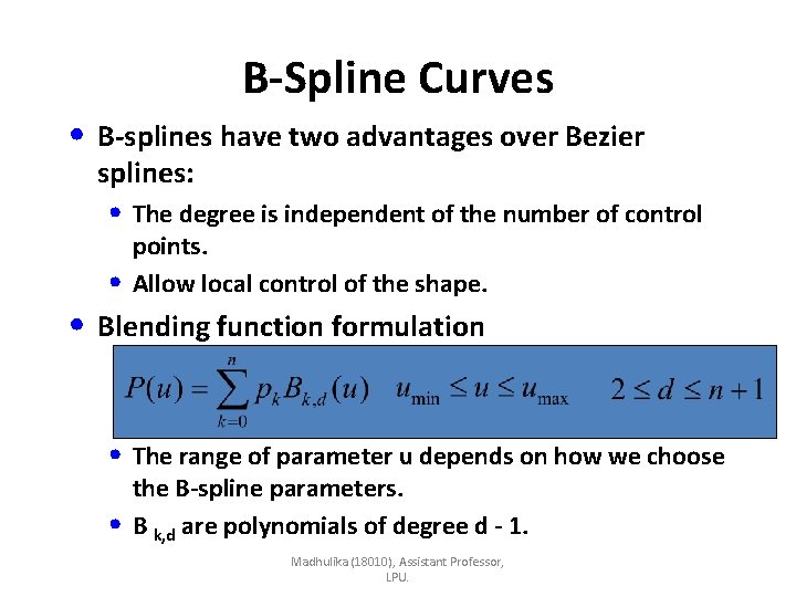
B-Spline Curves • B-splines have two advantages over Bezier splines: • The degree is independent of the number of control points. Allow local control of the shape. • • Blending function formulation • The range of parameter u depends on how we choose • the B-spline parameters. B k, d are polynomials of degree d - 1. Madhulika (18010), Assistant Professor, LPU.

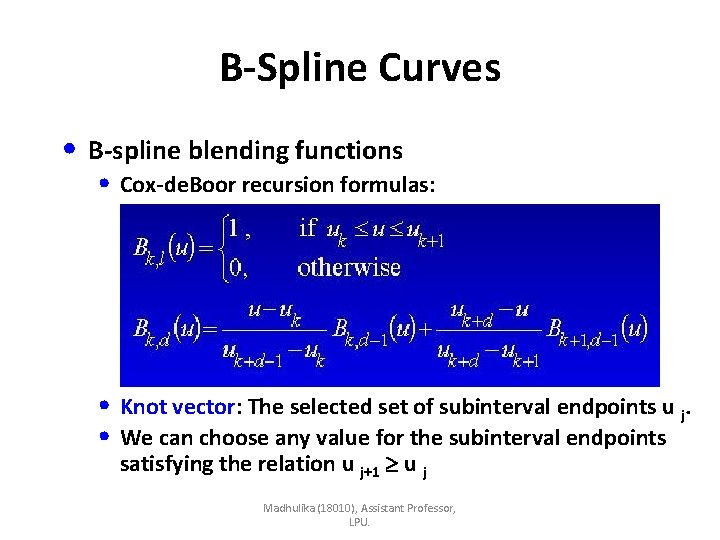
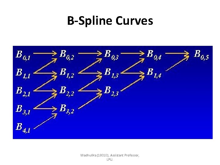
B-Spline Curves • B-spline blending functions • Cox-de. Boor recursion formulas: • Knot vector: The selected set of subinterval endpoints u j. • We can choose any value for the subinterval endpoints satisfying the relation u j+1 u j Madhulika (18010), Assistant Professor, LPU.

B-Spline Curves Madhulika (18010), Assistant Professor, LPU.

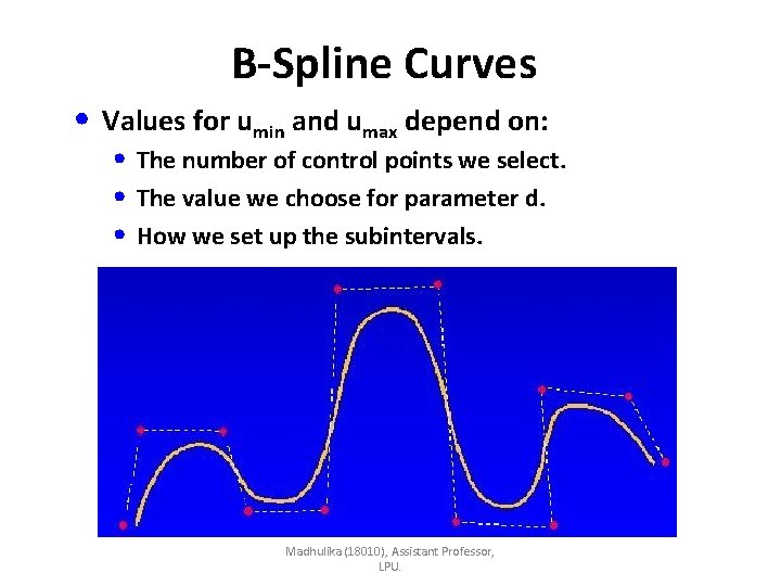
B-Spline Curves • Values for umin and umax depend on: • The number of control points we select. • The value we choose for parameter d. • How we set up the subintervals. Madhulika (18010), Assistant Professor, LPU.

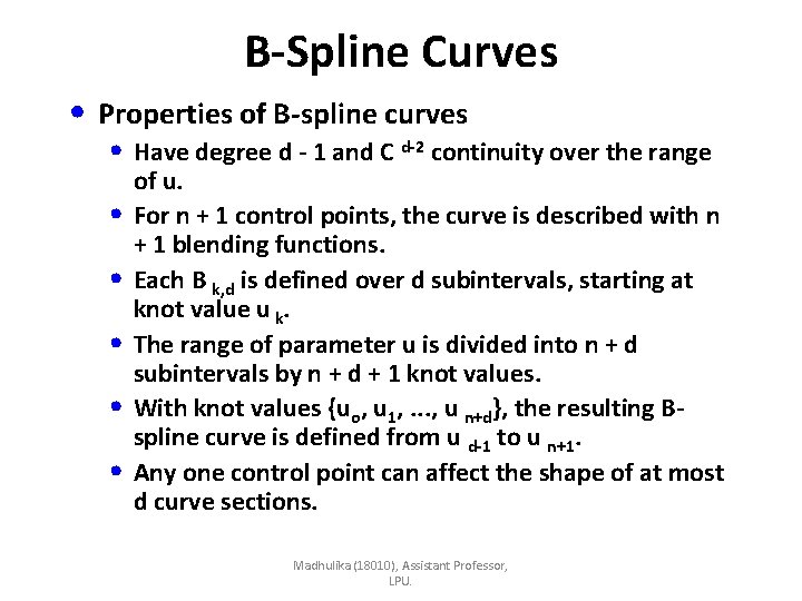
B-Spline Curves • Properties of B-spline curves • Have degree d - 1 and C d-2 continuity over the range • • • of u. For n + 1 control points, the curve is described with n + 1 blending functions. Each B k, d is defined over d subintervals, starting at knot value u k. The range of parameter u is divided into n + d subintervals by n + d + 1 knot values. With knot values {uo, u 1, . . . , u n+d}, the resulting Bspline curve is defined from u d-1 to u n+1. Any one control point can affect the shape of at most d curve sections. Madhulika (18010), Assistant Professor, LPU.

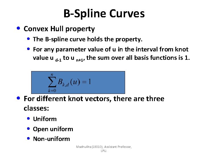
B-Spline Curves • Convex Hull property • The B-spline curve holds the property. • For any parameter value of u in the interval from knot value u d-1 to u n+1, the sum over all basis functions is 1. • For different knot vectors, there are three classes: • Uniform • Open uniform • Non-uniform Madhulika (18010), Assistant Professor, LPU.

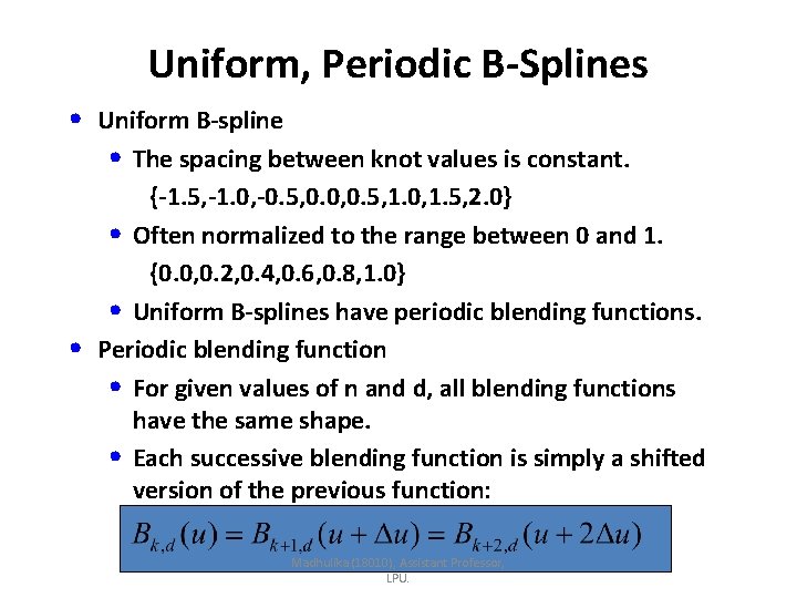
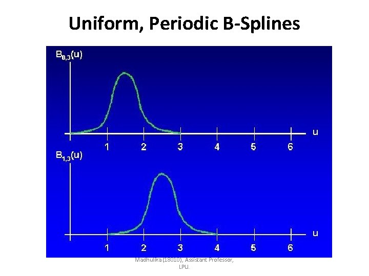
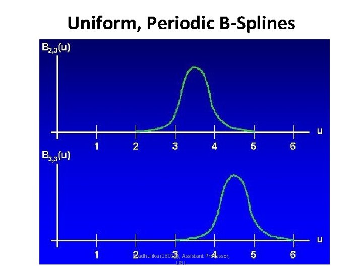
Uniform, Periodic B-Splines • Uniform B-spline • The spacing between knot values is constant. • {-1. 5, -1. 0, -0. 5, 0. 0, 0. 5, 1. 0, 1. 5, 2. 0} • Often normalized to the range between 0 and 1. {0. 0, 0. 2, 0. 4, 0. 6, 0. 8, 1. 0} • Uniform B-splines have periodic blending functions. Periodic blending function • For given values of n and d, all blending functions have the same shape. • Each successive blending function is simply a shifted version of the previous function: Madhulika (18010), Assistant Professor, LPU.

Uniform, Periodic B-Splines Madhulika (18010), Assistant Professor, LPU.

Uniform, Periodic B-Splines Madhulika (18010), Assistant Professor, LPU.

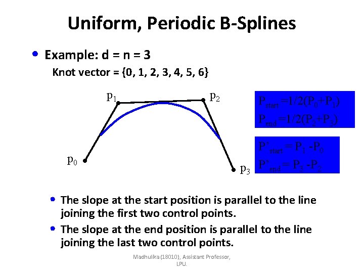
Uniform, Periodic B-Splines • Example: d = n = 3 Knot vector = {0, 1, 2, 3, 4, 5, 6} p 1 p 2 p 0 Pstart =1/2(P 0+P 1) Pend =1/2(P 2+P 3) p 3 P’start = P 1 -P 0 P’end = P 3 -P 2 • The slope at the start position is parallel to the line • joining the first two control points. The slope at the end position is parallel to the line joining the last two control points. Madhulika (18010), Assistant Professor, LPU.

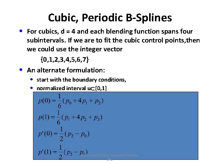
Cubic, Periodic B-Splines • For cubics, d = 4 and each blending function spans four • subintervals. If we are to fit the cubic control points, then we could use the integer vector {0, 1, 2, 3, 4, 5, 6, 7} An alternate formulation: • start with the boundary conditions, • normalized interval u [0, 1] Madhulika (18010), Assistant Professor, LPU.

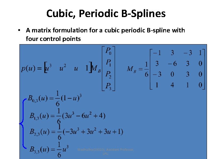
Cubic, Periodic B-Splines • A matrix formulation for a cubic periodic B-spline with four control points Madhulika (18010), Assistant Professor, LPU.

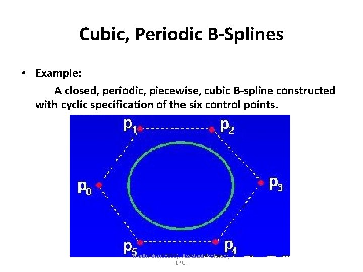
Cubic, Periodic B-Splines • Example: A closed, periodic, piecewise, cubic B-spline constructed with cyclic specification of the six control points. Madhulika (18010), Assistant Professor, LPU.

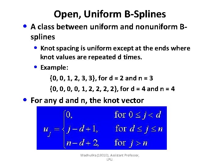
Open, Uniform B-Splines • A class between uniform and nonuniform B- splines • Knot spacing is uniform except at the ends where • knot values are repeated d times. Example: {0, 0, 1, 2, 3, 3}, for d = 2 and n = 3 {0, 0, 1, 2, 2}, for d = 4 and n = 4 • For any d and n, the knot vector Madhulika (18010), Assistant Professor, LPU.

Open, Uniform B-Splines • Characteristics are very similar to Bezier splines • When d = n + 1, open B-splines reduce to Bezier splines, all knot values are either 0, or 1. • Example: a cubic, open B-splines (d = 4) Knot vector = {0, 0, 1, 1, 1, 1} • An open B-spline passes through the first and last control points. • Specifying multiple control points at the same coordinate position pulls curve closer. Madhulika (18010), Assistant Professor, LPU.

Nonuniform B-Splines • Nonuniform B-splines • We can specify any values and intervals for the knot vector. • • {0, 1, 2, 3, 3, 4} {0, 2, 2, 3, 3, 6} {0, 0. 2, 0. 6, 0. 9, 1. 0} Provides increased flexibility in controlling a curve shape. Multiple knot values reduce the continuity by 1 for each repeat of a particular value. Madhulika (18010), Assistant Professor, LPU.

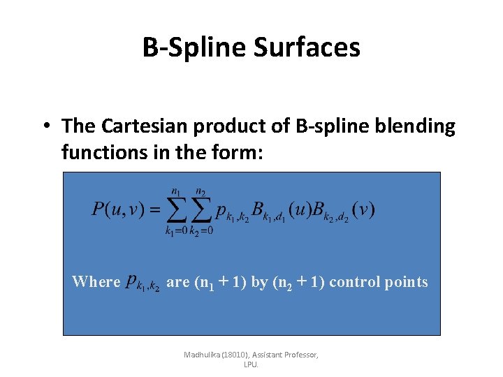
B-Spline Surfaces • The Cartesian product of B-spline blending functions in the form: Where are (n 1 + 1) by (n 2 + 1) control points Madhulika (18010), Assistant Professor, LPU.

Bezier vs. B-Spline Madhulika (18010), Assistant Professor, LPU.

Madhulika (18010), Assistant Professor, LPU.