Surface Water The Lane Diagram WATER SEDIMENT I

Surface Water

The Lane Diagram WATER SEDIMENT

I. Events During Precipitation A. Interception B. Stem Flow C. Depression Storage D. Hortonian Overland Flow E. Interflow F. Throughflow -> Return Flow G. Baseflow

II. Hydrograph A. General

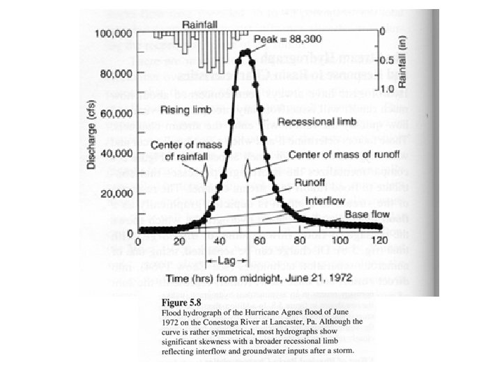
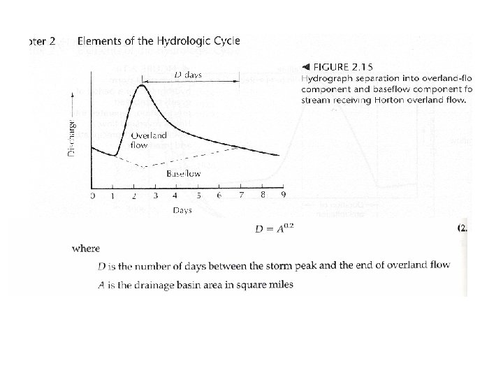
II. Hydrograph A. General B. Storm Hydrograph

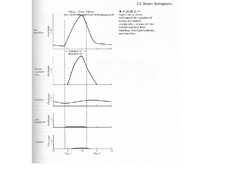
II. Hydrograph A. General B. Storm Hydrograph 1. Shape and Distribution of “events”

direct ppt. , runoff, baseflow, interflow

II. Hydrograph A. General B. Storm Hydrograph 1. Shape and Distribution of 2. Hydrograph Separation

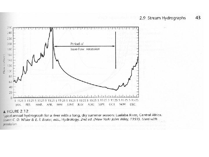
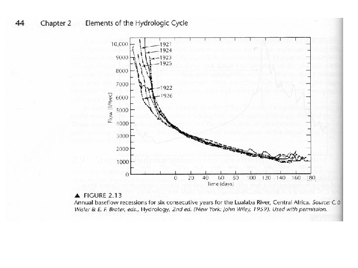
II. Hydrograph A. General B. Storm Hydrograph 1. Shape and Distribution of 2. Hydrograph Separation C. Predicting the rate of Baseflow Recession after a storm

vs.

Why care?

Predicting the rate of Baseflow Recession after a storm

Predicting the rate of Baseflow Recession after a storm

An example problem….

Gaining and Losing Streams…. .

III. Rainfall-Runoff Relationships

III. Rainfall-Runoff Relationships A. Time of Concentration

III. Rainfall-Runoff Relationships A. Time of Concentration “The time required for overland flow and channel flow to reach the basin outlet from the most distant part of the catchment”

III. Rainfall-Runoff Relationships A. Time of Concentration “The time required for overland flow and channel flow to reach the basin outlet from the most distant part of the catchment” tc = L 1. 15 7700 H 0. 38

III. Rainfall-Runoff Relationships A. Time of Concentration “The time required for overland flow and channel flow to reach the basin outlet from the most distant part of the catchment” tc = L 1. 15 7700 H 0. 38 tc = time of concentration (hr) L = length of catchment (ft) along the mainstream from basin mouth to headwaters (most distant ridge) H = difference in elevation between basin outlet and headwaters (most distant ridge)

L = 13, 385 ft H = 380 ft III. Rainfall-Runoff Relationships A. Time of Concentration tc = L 1. 15 example problem 7700 H 0. 38

L = 31, 385 ft H = 380 ft Tc = 0. 75 hrs, or 45 minutes tc = (13, 385) 1. 15 7700 (380) 0. 38 tc = time of concentration (hr) L = length of catchment (ft) along the mainstream from basin mouth to headwaters (most distant ridge) H = difference in elevation (ft) between basin outlet and headwaters (most distant ridge)

III. Rainfall-Runoff Relationships A. Time of Concentration B. Rational Equation

III. Rainfall-Runoff Relationships A. Time of Concentration B. Rational Equation If the period of ppt exceeds the time of concentration, then the Rational Equation applies

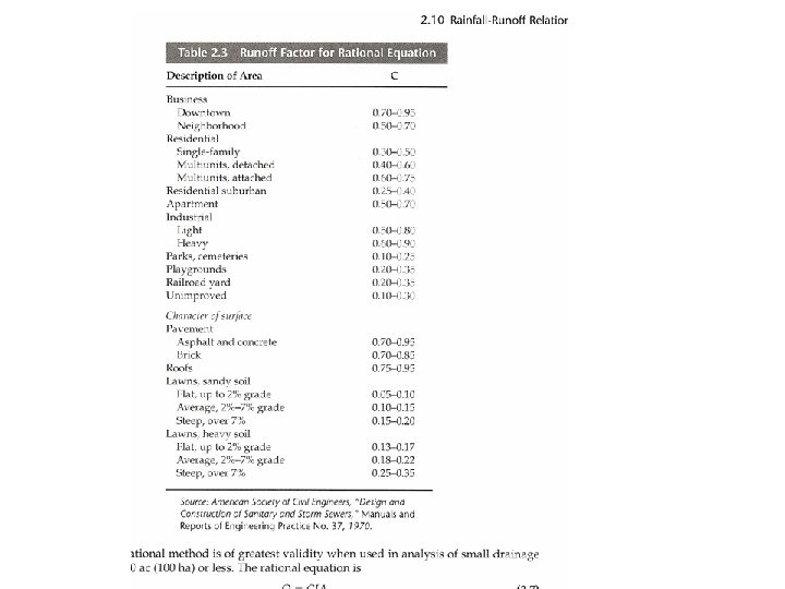
III. Rainfall-Runoff Relationships A. Time of Concentration B. Rational Equation Q=CIA

III. Rainfall-Runoff Relationships A. Time of Concentration B. Rational Equation Q=CIA Where Q=peak runoff rate (ft 3/s) C= runoff coeffic. I = ave ppt intensity (in/hr) A = drainage area (ac)

First: solve for time of concentration (“Duration”); THEN: solve for rainfall intensity for a given X year storm.

III. Rainfall-Runoff Relationships A. Time of Concentration B. Rational Equation example problem The drainage basin that ultimately flows past the JMU football stadium is dominated by an industrial park with flat roofed buildings, parking lots, shopping malls, and very little open area. The drainage basin has an area of 90 acres. Find the peak discharge during a storm that has a 25 year flood return interval.

First: solve for time of concentration (“Duration”); THEN: solve for rainfall intensity for a given X year storm. “ 45 minutes from previous exercise”

III. Rainfall-Runoff Relationships A. Time of Concentration B. Rational Equation example problem The drainage basin that ultimately flows past the JMU football stadium is dominated by an industrial park with flat roofed buildings, parking lots, shopping malls, and very little open area. The drainage basin has an area of 90 acres. Find the peak discharge during a storm that has a 25 year flood return interval. Q = ci. A

III. Rainfall-Runoff Relationships A. Time of Concentration B. Rational Equation example problem The drainage basin that ultimately flows past the JMU football stadium is dominated by an industrial park with flat roofed buildings, parking lots, shopping malls, and very little open area. The drainage basin has an area of 90 acres. Find the peak discharge during a storm that has a 25 year flood return interval. Q = ci. A Q = (0. 85)*(2. 5 in/hr)*(90 acres)

III. Rainfall-Runoff Relationships A. Time of Concentration B. Rational Equation example problem The drainage basin that ultimately flows past the JMU football stadium is dominated by an industrial park with flat roofed buildings, parking lots, shopping malls, and very little open area. The drainage basin has an area of 90 acres. Find the peak discharge during a storm that has a 25 year flood return interval. Q = 191. 3 ft 3/s

III. Rainfall-Runoff Relationships A. Time of Concentration B. Rational Equation example problem The drainage basin that ultimately flows past the JMU football stadium is dominated by an industrial park with flat roofed buildings, parking lots, shopping malls, and very little open area. The drainage basin has an area of 90 acres. Find the peak discharge during a storm that has a 25 year flood return interval. Calculate the mean velocity if the cross sectional area of the channel is 40 ft 2.

III. Rainfall-Runoff Relationships A. Time of Concentration B. Rational Equation example problem An industrial park with flat roofed buildings, parking lots, and very little open area has a drainage basin area of 90 acres. The 25 year flood has an intensity of 2 in/hr. Find the peak discharge during the storm. Calculate the mean velocity if the cross sectional area of the channel is 40 ft 2. Discharge = Velocity x Area

III. Rainfall-Runoff Relationships A. Time of Concentration B. Rational Equation example problem An industrial park with flat roofed buildings, parking lots, and very little open area has a drainage basin area of 90 acres. The 25 year flood has an intensity of 2 in/hr. Find the peak discharge during the storm. Calculate the mean velocity if the cross sectional area of the channel is 40 ft 2. Discharge = Velocity x Area 191. 3 ft 3/s = 40 ft 2 * V V = 4. 8 ft/s

Calculate the mean velocity if the cross sectional area of the channel is 40 ft 2. Discharge = Velocity x Area 191. 3 ft 3/s = 40 ft 2 * V V = 4. 8 ft/s or 146. 3 cm/s If the channel is made of fine sand, will it remain stable?

Hjulstrom Diagram 146. 3 cm/s 0. 10 -0. 25 mm (fine sand) size range

III. Measurement of Streamflow

III. Measurement of Streamflow A. Direct Measurements B. Indirect Measurements

III. Measurement of Streamflow A. Direct Measurements

III. Measurement of Streamflow A. Direct Measurements 1. Price /Gurley/Marsh-Mc. Birney Current Meters

III. Measurement of Streamflow A. Direct Measurements 1. Price or Gurley Current Meter 2. Weirs

Weirs rectangular Q = 1. 84 (L – 0. 2 H)H 3/2 Where L = length of weir crest (m), H = ht of backwater above weir crest (m), Q = m 3/s *note: eq. 2. 16 B in Fetter is incorrect (exponent is 3/2 as shown above)

Weirs V notch Q=1. 379 H 5/2 Where H = ht of backwater above weir crest (m) Q = m 3/s

III. Measurement of Streamflow B. Indirect Measurements

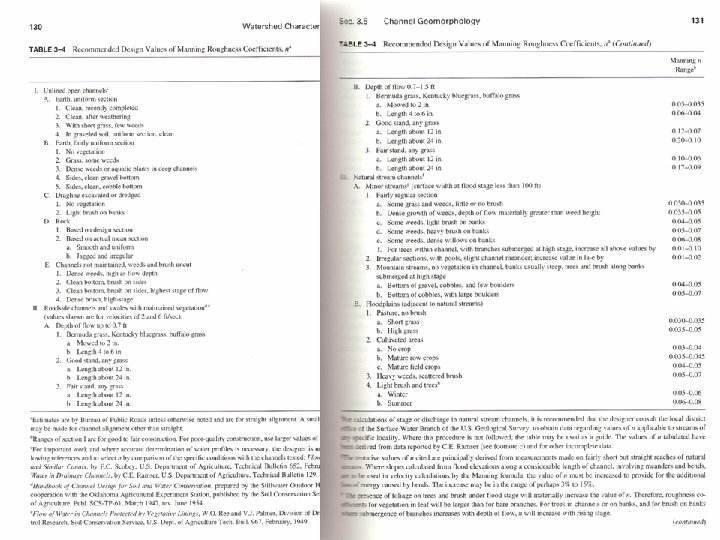
III. Measurement of Streamflow B. Indirect Measurements 1. Manning Equation V = R 2/3 S ½ n Where V = average flow velocity (m/s) R = hydraulic radius (m) S = channel slope (unitless) n = Manning roughness coefficient

1. Manning Equation V = R 2/3 S ½ n Where V = average flow velocity (m/s) R = hydraulic radius (m) S = channel slope (unitless) n = Manning roughness coefficient R = A/P A = Area (m 2) P = Wetted Perimeter (m)

1. Manning Equation If using English units…. . V = 1. 49 * R 2/3 S ½ n Where V = average flow velocity (ft/s) R = hydraulic radius (ft) S = channel slope (unitless) n = Manning roughness coefficient R = A/P A = Area (ft 2) P = Wetted Perimeter (ft)

V = R 2/3 S ½ n If Q = V * A, then Q = A R 2/3 S ½ n Where Q = average flow discharge (m 3/s) A = area of channel (m 2) R = hydraulic radius (m) S = channel slope (unitless) n = Manning roughness coefficient R = A/P A = Area P = Wetted Perimeter

Q = A R 2/3 S ½ N Where Q = average flow discharge A = area of channel r = hydraulic radius s = channel slope (unitless) n = Manning roughness coefficient R = A/P A = Area P = Wetted Perimeter Example Problem: A flood that occurred in a mountain stream comprised of cobbles, pebbles, and few boulders creates a high water mark of 3 meters above the bottom of the channel, and temporarily expands the channel width to 6 m. The slope of the water surface is 100 meters of drop per 1 km of distance. Determine V in m/s Determine Q in m 3/s

B. Indirect Measurements 1. Manning Equation 2. Super. Elevation Method 3. Measurement of Cobbles

B. Indirect Measurements 1. Manning Equation 2. Super. Elevation Method

B. Indirect Measurements 1. Manning Equation 2. Super. Elevation Method Q = A(Rc*g*cos. S * tanΘ) ½ Q = discharge, A = average radial cross section in the bend, Rc= radius of curvature S = slope of channel (degrees) Θ = angle between high water marks on opposite banks (degrees) Example Problem:

B. Indirect Measurements 3. Measurement of Cobbles

B. Indirect Measurements 3. Measurement of Cobbles The “Costa Equation” V = 0. 18 d 0. 49 Where V =m/s, d=mm where 50 < d < 3200 mm Measure the 5 largest boulders, intermediate axis, take the average

B. Indirect Measurements 3. Measurement of Cobbles V = 0. 18 d 0. 49 Where V =m/s, d=mm and 50 < d < 3200 mm Measure the 5 largest boulders, intermediate axis And hc = {V {4. 5*{(S + 0. 001)0. 17}} }1. 5 Where V = velocity, in m/s S energy slope (decimal form) hc = competent flood depth (m) Example Problem: Average of five largest boulders: 3. 2 m x 2. 3 m x 1. 6 m Average slope = 5. 5 degrees Find: average velocity and depth of flow

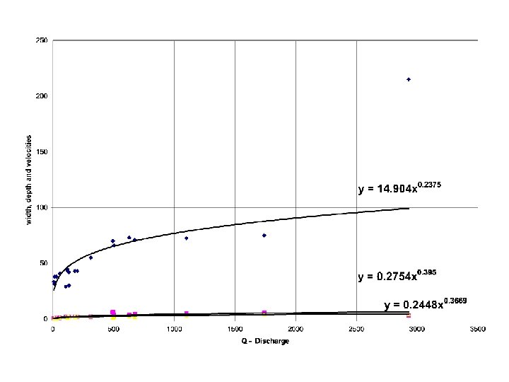
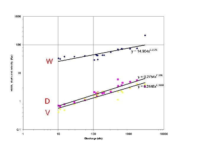
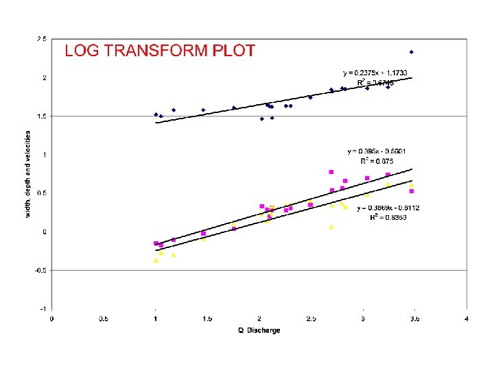
V. Hydraulic Geometry A. The relationships Q = V*A Q=V*w*d w = a. Qb d = c. Q f v = k. Q m

V. Hydraulic Geometry A. The relationships B. “at a station” C. “distance downstream”

A. Hydraulic Geometry “at a station trends” M = 0. 26 M = 0. 4 M = 0. 34

A. Hydraulic Geometry M = 0. 5 M = 0. 4 “distance downstream trends” M = 0. 1

Distance Downstream

VI. Flood Frequency Analysis B. Flow Duration Curves

VI. Flood Frequency Analysis Flood recurrence interval (R. I. ) use Weibull Method - calculates the R. I. by taking the average time between 2 floods of equal or greater magnitude. RI = (n + 1) / m where n is number of years on record, m is magnitude of given flood

VI. Flood Frequency Analysis What does this mean? ? ? the curve estimates the magnitude of a flood that can be expected within a specified period of time The probability that a flow of a given magnitude will occur during any year is P = 1/RI. EX: a 50 year flood has a 1/50 th chance, or 2 percent chance of occurring in any given year.

VI. Flood Frequency Analysis For multiple years: q = 1 - ( 1 -1/RI)n where q = probability of flood with RI with a specified number of years n

VI. Flood Frequency Analysis For multiple years: q = 1 - ( 1 -1/RI)n where q = probability of flood with RI with a specified number of years n EX: a 50 year flood has an 86% chance of occurring over 100 years Example Problem: Determine the water height during a 100 year storm at the Harrison Gaging Station near Grottoes, Virginia.

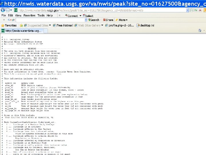
VI. Flood Frequency Analysis Example Problem: Determine the water height during a 100 year storm at the Harrison Gaging Station near Grottoes, Virginia. Method: • Access data at www. usgs. gov; select water tab • Select “water watch” under ‘streams, lakes, rivers’ option • Choose the current stream flow map, your state and the respective station location • Open station page by clicking on the station number • Select “surface water - peak streamflow” option • Choose ‘tab separated file’ format • Highlight, copy, and paste (special) your data to Excel for analysis.

VI. Flood Frequency Analysis Example Problem: Determine the water height during a 100 year storm at the Harrison Gaging Station near Grottoes, Virginia. Method (continued): • Clean up data so that only ‘Year’ , ‘Q’, and ‘Gage Ht. ’ are present • Sort data based on Q in descending order • Add magnitude (m) ranking (highest = 1) • Add RI formula, where RI = (n+1)/m • Create graph depicting RI vs. Q • Create graph of Q vs. Gage Ht. • Determine Gage Height with respect to the given RI

Magnitud Year Q (cfs) Gage Ht (ft) e RI (yrs) 9/6/1996 28900 15. 57 1 73. 0 11/4/1985 28100 15. 47 2 36. 5 10/15/1942 23100 17. 2 3 24. 3 9/19/2003 22000 14. 41 4 18. 3 6/21/1972 21300 15. 25 5 14. 6 1924 -05 -00 21000 16. 6 6 12. 2 9/6/1979 16200 13. 47 7 10. 4 10/5/1972 15300 13. 24 8 9. 1 3/18/1936 12600 13. 07 9 8. 1 3/19/1975 12400 12. 2 10 7. 3 9/28/2004 12300 12. 26 11 6. 6 8/16/1940 12100 12. 91 12 6. 1 4/17/2011 11900 12. 15 13 5. 6 4/26/1937 11700 13 14 5. 2 9/18/1945 11300 12. 8 15 4. 9 8/20/1969 11100 12. 72 16 4. 6 1/25/2010 11100 11. 9 17 4. 3 11/29/2005 10900 11. 84 18 4. 1 3/19/1983 10300 11. 44 19 3. 8 9/20/1928 10100 11. 9 20 3. 7 2/17/1998 10000 11. 59 21 3. 5 4/22/1992 9840 11. 8 22 3. 3 5/30/1971 9460 11. 93 23 3. 2 10/17/1932 8700 11. 5 24 3. 0 12/1/1934 8340 11. 3 25 2. 9 9/19/1944 8340 11. 33 26 2. 8 10/9/1976 8250 10. 62 27 2. 7 2/14/1984 8250 10. 6 28 2. 6 4/17/1987 8120 11. 08 29 2. 5 6/18/1949 7980 11. 06 30 2. 4 1/26/1978 7800 10. 38 31 2. 4

35000 30000 Discharge (cfs) 25000 20000 15000 10000 5000 0 10. 0 Recurrence Interval (yrs) 100. 0

Discharge (cfs) Gage Height (ft)

VI. Flood Frequency B. Flow Duration Curves

VI. Flood Frequency B. Flow Duration Curves “shows the percentage of time that a given flow of a stream will be equaled or exceeded. ”

B. Flow Duration Curves “shows the percentage of time that a given flow of a stream will be equaled or exceeded. ” P = * m * (100) n+1

B. Flow Duration Curves “shows the percentage of time that a given flow of a stream will be equaled or exceeded. ” P = * m * (100) n+1

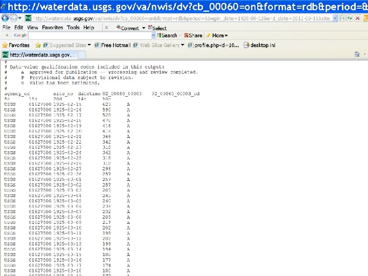
VI. Flood Frequency B. Flow Duration Example Problem: Determine the discharge that can be expected 80% of the time at the Harrison Gaging Station near Grottoes, Virginia. Method: • Access data at www. usgs. gov; select water tab • Select “water watch” under ‘streams, lakes, rivers’ option • Choose the current stream flow map, your state and the respective station location • Open station page by clicking on the station number • Select “daily data” option, • Then click ‘mean discharge’ option • Choose the earliest date of record through ‘present’ • Choose ‘tab separated file’ format, and select ‘go’ • Highlight, copy, and paste (special) your data to Excel for analysis.

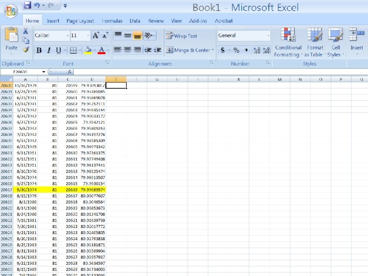
VI. Flood Frequency Analysis Example Problem: Determine the discharge that can be expected 80% of the time at the Harrison Gaging Station near Grottoes, Virginia. Method (continued): • Clean up data so that only ‘Year’ , ‘Q’, and ‘Gage Ht. ’ are present • Sort data based on Q in descending order • Add magnitude (m) ranking (highest = 1) • Add P formula, where P = m/(n+1) • Pick out desired probability value, and record the respective discharge

P = * m * 100 n+1

How much water would this value of discharge y for a full day?

How much water would this value of discharge y for a full day? 81 ft 3 * 3600 s * 24 hr = 6, 998, 400 ft 3 of wate s 1 hr 1 d

V. Sediment Transport A. Shear Stress τc = critical boundary shear stress hc = minimal water depth required for flow ρw = water density (assume 1. 00 g/cm 3) g = gravitational acceleration (981 cm/s 2) S = slope (decimal e. g. , meters per meters)

V. Sediment Transport A. Shear Stress τc = hc ρw g S τc = critical boundary shear stress (force per unit area) (g/cm-s 2) hc = minimal water depth required for flow (cm) ρw = water density (assume 1. 00 g/cm 3) g = gravitational acceleration (981 cm/s 2) S = slope (decimal, e. g. , meters per meters)

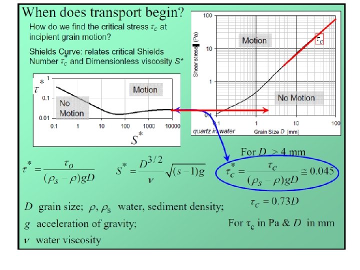
V. Sediment Transport 1. Shear Stress 2. The Shields Equation τc = hc ρw g S τc = τ*c (ρs – ρw)g. D 50 τc = critical boundary shear stress hc = minimal water depth required for flow ρs, ρw = grain density (assume 2. 65 g/cm 3) and water density g = gravitational acceleration (981 cm/s 2) D 50 = median bed material grain size τ*c = dimensionless critical shear stress (the Shields number) 0. 03 for sand, 0. 047 for gravel

V. Sediment Transport 1. Shear Stress τc = hc ρw g S 2. Shields Equation τc = τ*c (ρs – ρw)g. D 50 OR hc =(ρs – ρw) τ*c D 50 ρw. S τc = critical boundary shear stress hc = minimal water depth required for flow ρs, ρw = grain density (assume 2. 65 g/cm 3) and water density g = gravitational acceleration (981 cm/s 2) D 50 = median bed material grain size τ*c = dimensionless critical shear stress (the Shields number) 0. 03 for sand, 0. 047 for gravel

Problem: A gravel bed stream of slope 2 m per 1 km has a median grain size of 60 mm. Caculate: 1) the critical shear stress required for bedload mobilization; 2) The critical water depth to initiate motion τc = hc ρw g S τc = τ*c (ρs – ρw)g. D 50 OR hc =(ρs – ρw) τ*c D 50 ρw. S τc = critical boundary shear stress hc = minimal water depth required for flow ρs, ρw = grain density (assume 2. 65 g/cm 3) and water density g = gravitational acceleration (981 cm/s 2) D 50 = median bed material grain size τ*c = dimensionless critical shear stress (the Shields number) 0. 03 for sand, 0. 047 for gravel