Supporting OnDemand Elasticity in Distributed Graph Processing Mayank

Supporting On-Demand Elasticity in Distributed Graph Processing Mayank Pundir*, Manoj Kumar, Luke M. Leslie, Indranil Gupta, Roy H. Campbell University of Illinois at Urbana-Champaign *Facebook (work done at UIUC)

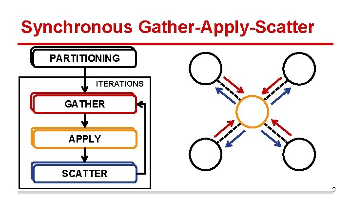
Synchronous Gather-Apply-Scatter PARTITIONING ITERATIONS GATHER APPLY SCATTER 2

Background: Existing Systems • Systems are typically configured with a static set of servers. • • Power. Graph [Gonzalez et al. OSDI 2012] Giraph [Ching et al. , VLDB 2015] Pregel [Malewicz et al. SIGMOD 2010] LFGraph [Hoque et al. TRIOS 2013] • Consequently, these systems lack the flexibility to scale-out/in during computation. 3

Background: Graph Partitioning • Current mechanisms partition the entire graph across a fixed set of servers. • Partitioning occurs once at the start of computation. • Supporting elasticity requires an incremental approach to partitioning. • We must repartition during computation as servers leave and join. 4

Background: Graph Partitioning • We assume hash-based vertex partitioning. • Use consistent hashing. • Vertex assigned to server with ID = hash(v) % N • Recent studies [Hoque et al 2013] have shown hash -based vertex partitioning: • Involves the least amount of overhead. • Performs well. 5

Our Contribution • We present and analyze two techniques to achieve scale-out/in in distributed graph processing systems. 1. Contiguous Vertex Repartitioning (CVR). 2. Ring-based Vertex Repartitioning (RVR). • We have implemented our techniques in LFGraph. • Experiments show performance within 9% and 21% of optimum for scale-out and scale-in operations. 6

Key Questions 1. How (and what) to migrate? • • How should vertices be migrated to minimize network overhead? What vertex data must be migrated? 2. When to migrate? • At what point during computation should migration start/end? 7

How (and What) to Migrate? • Assumption: hashed vertex space is divided into equi-sized partitions. • Key Problem: upon scale-out/in, how do we assign new equi-sized partitions to servers? • Goal: minimize network overhead. 8

How (and What) to Migrate? Servers (4) Before S 1 [V 1, V 25] [V 21, V 25] After S 1 [V 1, V 20] S 2 [V 25, V 50] [V 41, V 50] S 2 [V 21, V 40] S 3 [V 51, V 75] [V 61, V 75] S 3 [V 41, V 60] S 4 [V 76, V 100] [V 81, V 100] S 4 [V 61, V 80] Total transfer: 5 + 10 + 15 + 20 = 50 vertices S 5 [V 81, V 100] Servers (5) 9

How (and What) to Migrate? Servers (4) Before S 1 [V 1, V 25] [V 21, V 25] After S 1 [V 1, V 20] S 2 [V 25, V 50] [V 41, V 50] S 2 [V 21, V 40] S 3 [V 51, V 75] [V 51, V 60] S 3 [V 41, V 60] S 4 [V 76, V 100] [V 76, V 80] S 4 [V 61, V 80] Total transfer: 5 + 10 + 5 = 30 vertices S 5 [V 81, V 100] Servers (5) 10

How (and What) to Migrate? CVR: Contiguous Vertex Repartitioning • Intuition: Reduce to min cost graph matching problem and utilize an efficient heuristic. • Can use O(N) greedy algorithm due to contiguity of partitions. 11

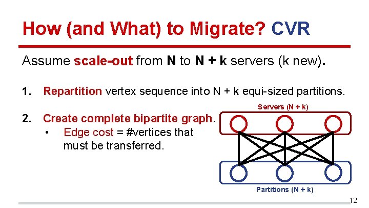
How (and What) to Migrate? CVR Assume scale-out from N to N + k servers (k new). 1. Repartition vertex sequence into N + k equi-sized partitions. Servers (N + k) 2. Create complete bipartite graph. • Edge cost = #vertices that must be transferred. Partitions (N + k) 12

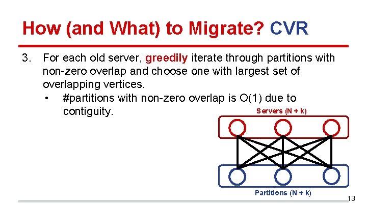
How (and What) to Migrate? CVR 3. For each old server, greedily iterate through partitions with non-zero overlap and choose one with largest set of overlapping vertices. • #partitions with non-zero overlap is O(1) due to Servers (N + k) contiguity. Partitions (N + k) 13

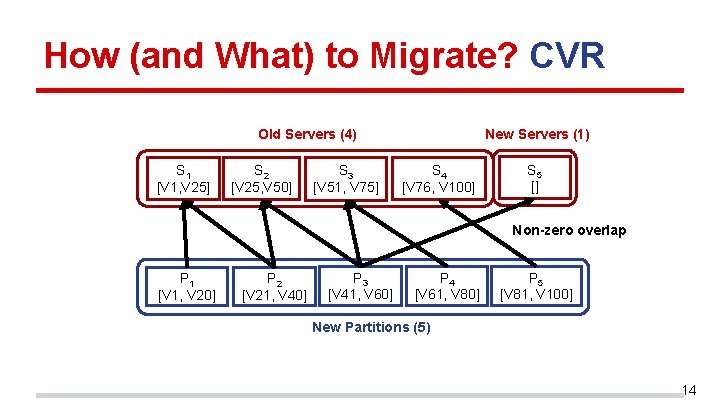
How (and What) to Migrate? CVR New Servers (1) Old Servers (4) S 1 [V 1, V 25] S 2 [V 25, V 50] S 3 [V 51, V 75] S 4 [V 76, V 100] S 5 [] Non-zero overlap P 1 [V 1, V 20] P 2 [V 21, V 40] P 3 [V 41, V 60] P 4 [V 61, V 80] P 5 [V 81, V 100] New Partitions (5) 14

How (and What) to Migrate? CVR Given a load-balanced system, we prove that to minimize network traffic and preserve load balance: • Scale-out: joining server placed in the middle of list. • • I. e. , insert after SN/2. Scale-in: leaving server must be middle server in list. • I. e. , remove S(N+1)/2. 15

Can we do better? Problems: With CVR, we experience (1) imbalanced load across servers when transferring vertices, (2) many servers involved in each operation. • In the previous example, servers close to the middle transferred twice as many vertices. Question: Can we find a way to provide better load balance and minimize the number of affected servers? 16

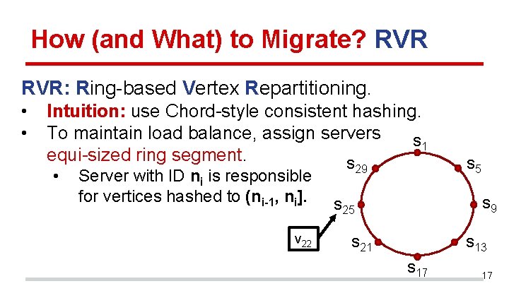
How (and What) to Migrate? RVR: Ring-based Vertex Repartitioning. • • Intuition: use Chord-style consistent hashing. To maintain load balance, assign servers s 1 equi-sized ring segment. s • Server with ID ni is responsible for vertices hashed to (ni-1, ni]. v 22 29 s 5 s 9 s 25 s 21 s 13 s 17 17

How (and What) to Migrate? RVR General process: • Scale-out: joining server splits successor’s segment. • • I. e. , ni takes (ni-1, ni] from ni+1. Scale-in: leaving server gives segment to successor. • I. e. , ni gives (ni-1, ni] to ni+1. Scale-out/in operation with k servers affects at most k other servers. 18

How (and What) to Migrate? RVR Given a load-balanced system… • Scale-out: spread out affected portions over the ring. • • • For �k/N�rounds, assign N servers each to a disjoint old partition. ≤ N servers being added => V/2 N vertices transferred per addition. Otherwise, only minimax if m-1< k/N ≤ m, where m is the maximum number of new servers added to an old partition. 19

How (and What) to Migrate? RVR Given a load-balanced system… • Scale-in: remove alternating servers. • • ≤ N/2 servers being removed => V/N vertices transferred per removal. Otherwise, only minimax if (m-1)/m < k/N ≤ m/(m + 1), where m is the maximum number of servers removed from an old partition. 20

LFGraph: a brief overview • Graph is partitioned (equi-sized) among servers. • Partitions further divided among worker threads. • Into vertex groups (one per thread). • Centralized barrier server for synchronization. • Communication occurs via pub-sub mechanism. • Servers subscribe to in-neighbors of vertices. 21

When to Migrate? • Must decide when to migrate vertices to minimize interference with ongoing computation. • Migration includes static data and dynamic data. • • Static data: vertex IDs, neighbor IDs, edge values. Dynamic data: vertex states. 22

When to Migrate? • Possible solution: migrate everything during synchronization interval between iterations. • Problem: migrating both static and dynamic data during this interval is very wasteful. • • Migration might only involve a few servers. Static data doesn’t change – can be migrated at any point. 23

When to Migrate? • Solution: migrate static data in the background, and dynamic data during synchronization. • Migration is merged with the scatter phase to further reduce overhead. 24

LFGraph Optimizations Parallel Migration: • If two servers are running the same number of threads, there is a one-to-one correspondence between ring segments (and thus vertex groups). • Thus, we can transfer data directly and in parallel between corresponding threads. 25

LFGraph Optimizations RVR Optimizations: 1. Modified scatter phase transfers vertex values from servers to successors in parallel w/reconfiguration. 2. During scale-in, servers quickly rebuild subscription lists by appending leaving server’s list to successors. 26

LFGraph Optimizations Pre-Building Subscription Lists: • Allow servers to receive information in background from barrier server about joining/leaving servers. • Hence, can start building subscription lists before cluster reconfiguration. 27

Experimental Setup • Up to 30 servers, each with 16 GB RAM, 8 CPUs. • Twitter Graph: 41. 65 M vertices, 1. 47 B edges. • Algorithms: Page. Rank, SSSP, MSSP, Connected Components, K-means. • Infinite Bandwidth (IB) baseline: repartitioning under infinite network bandwidth. • • Assume cluster converges immediately to new size. Measure overhead as the increase in iteration time 28

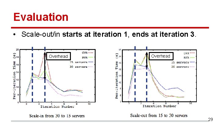
Evaluation • Scale-out/in starts at iteration 1, ends at iteration 3. Overhead 29

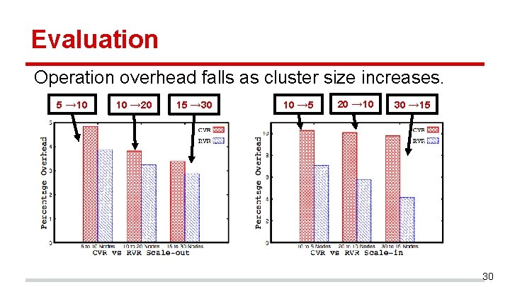
Evaluation Operation overhead falls as cluster size increases. 5 → 10 10 → 20 15 → 30 10 → 5 20 → 10 30 → 15 30

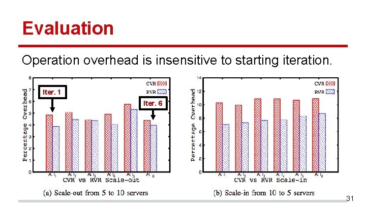
Evaluation Operation overhead is insensitive to starting iteration. Iter. 1 Iter. 6 31

Evaluation For Page. Rank: • RVR: overhead vs. optimal is <6% for scale-out, <8% for scale-in. • CVR: overhead vs. optimal is <6% for scale-out, <11% for scale-in. 32

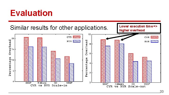
Evaluation Similar results for other applications. Lower execution time => higher overhead 33

Evaluation For other algorithms: • RVR: overhead vs. optimal is <8% for scale-out, <16% for scale-in. • CVR: overhead vs. optimal is <9% for scale-out, <21% for scale-in. 34

Conclusions • We have proposed two techniques to enable ondemand elasticity in distributed graph processing systems: CVR and RVR. • We have integrated CVR and RVR into LFGraph. • Experiments show that our approaches incur <9% overhead for scale-out, <21% for scale-in. http: //dprg. cs. uiuc. edu http: //srg. cs. illinois. edu 35