Support Vector Regression David R Musicant and O

Support Vector Regression David R. Musicant and O. L. Mangasarian International Symposium on Mathematical Programming Thursday, August 10, 2000 http: //www. cs. wisc. edu/~musicant

Outline l Robust Regression – – l Huber M-Estimator loss function New quadratic programming formulation Numerical comparisons Nonlinear kernels Tolerant Regression – New formulation of Support Vector Regression (SVR) – Numerical comparisons – Massive regression: Row-column chunking l Conclusions & Future Work 2

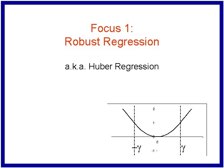
Focus 1: Robust Regression a. k. a. Huber Regression -g g

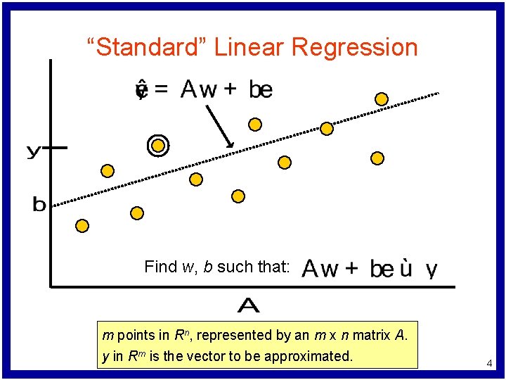
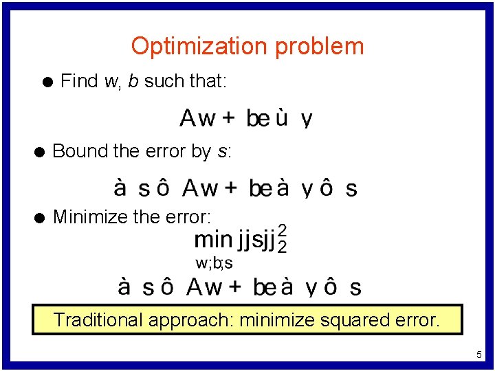
“Standard” Linear Regression Find w, b such that: m points in Rn, represented by an m x n matrix A. y in Rm is the vector to be approximated. 4

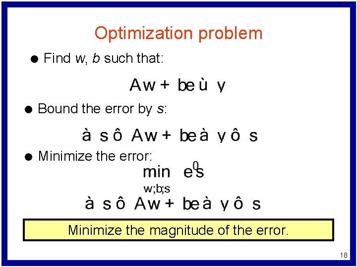
Optimization problem l Find w, b such that: l Bound the error by s: l Minimize the error: Traditional approach: minimize squared error. 5

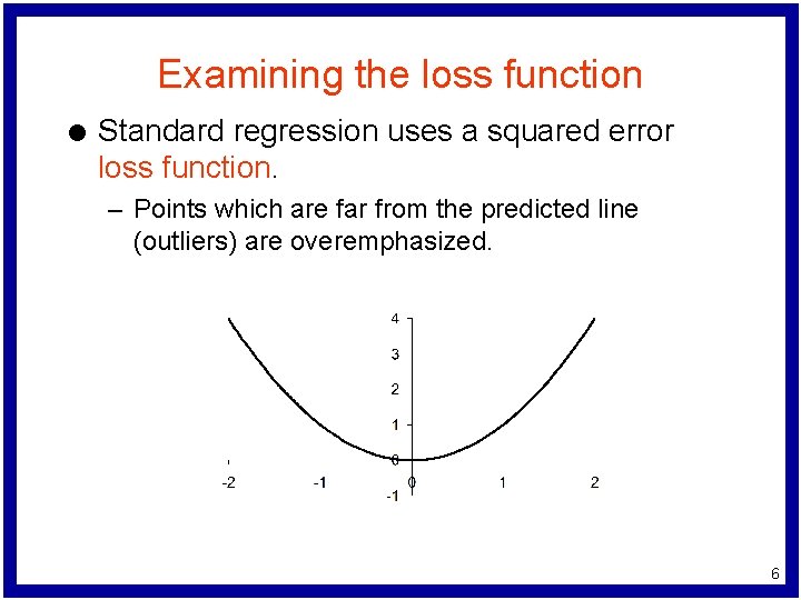
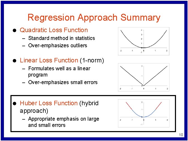
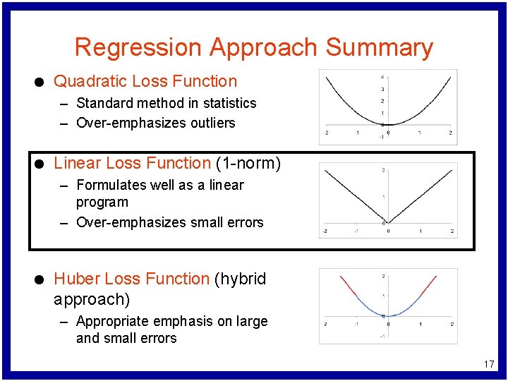
Examining the loss function l Standard regression uses a squared error loss function. – Points which are far from the predicted line (outliers) are overemphasized. 6

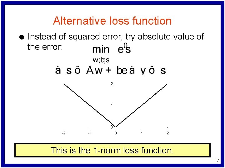
Alternative loss function l Instead of squared error, try absolute value of the error: This is the 1 -norm loss function. 7

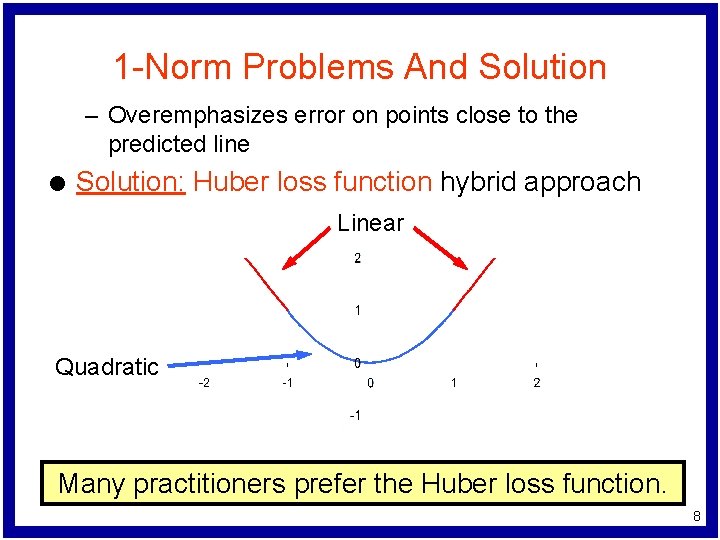
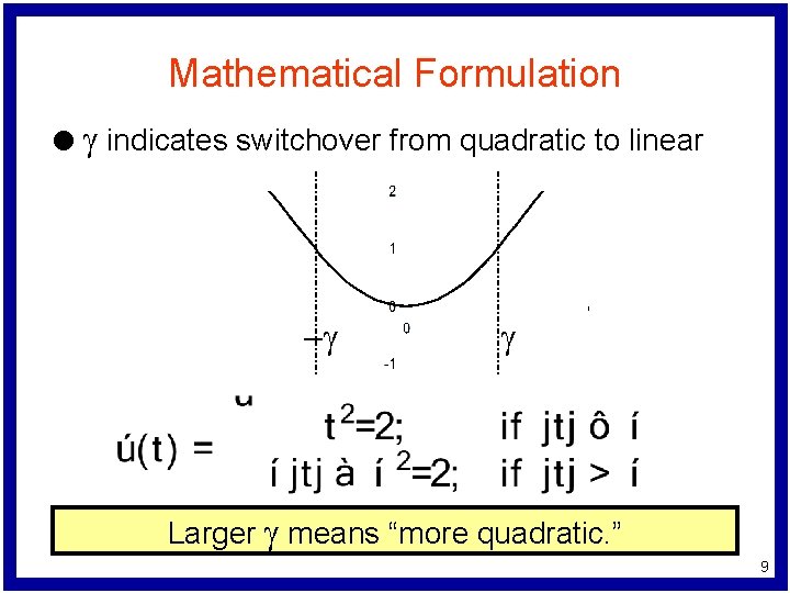
1 -Norm Problems And Solution – Overemphasizes error on points close to the predicted line l Solution: Huber loss function hybrid approach Linear Quadratic Many practitioners prefer the Huber loss function. 8

Mathematical Formulation l g indicates switchover from quadratic to linear -g g Larger g means “more quadratic. ” 9

Regression Approach Summary l Quadratic Loss Function – Standard method in statistics – Over-emphasizes outliers l Linear Loss Function (1 -norm) – Formulates well as a linear program – Over-emphasizes small errors l Huber Loss Function (hybrid approach) – Appropriate emphasis on large and small errors 10

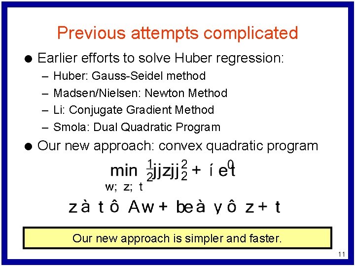
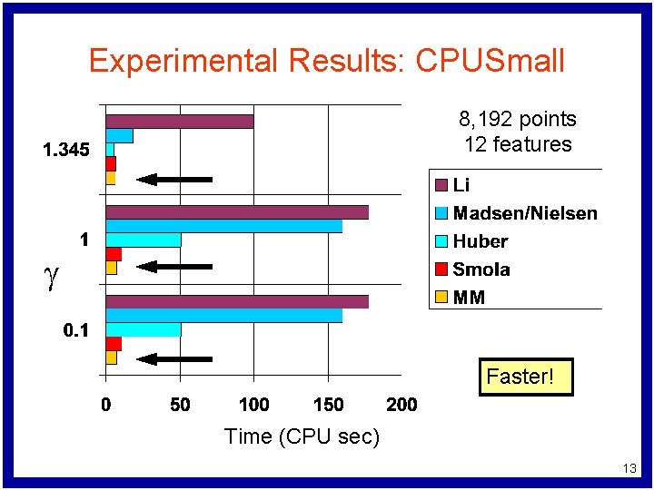
Previous attempts complicated l Earlier efforts to solve Huber regression: – – l Huber: Gauss-Seidel method Madsen/Nielsen: Newton Method Li: Conjugate Gradient Method Smola: Dual Quadratic Program Our new approach: convex quadratic program Our new approach is simpler and faster. 11

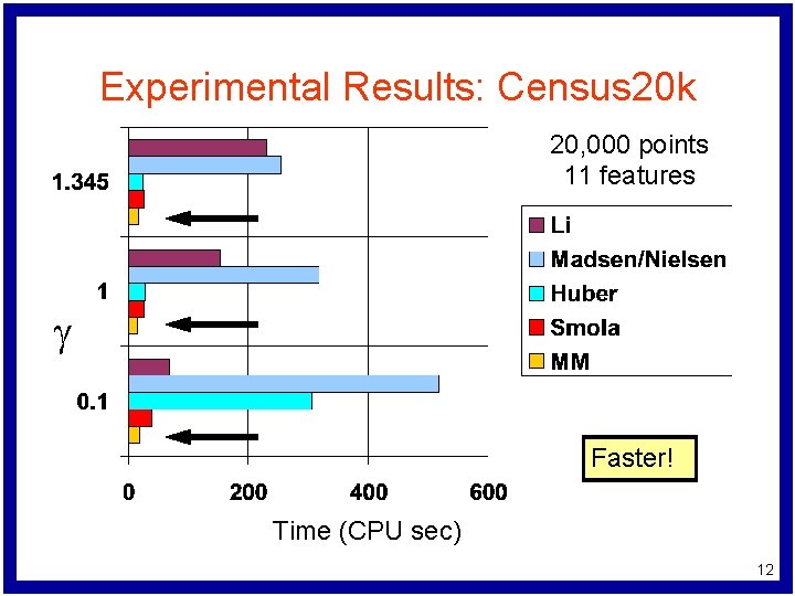
Experimental Results: Census 20 k 20, 000 points 11 features g Faster! Time (CPU sec) 12

Experimental Results: CPUSmall 8, 192 points 12 features g Faster! Time (CPU sec) 13

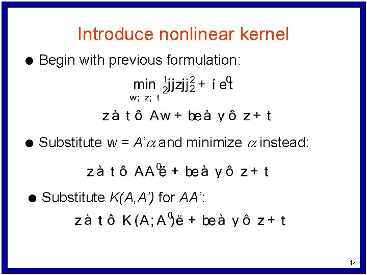
Introduce nonlinear kernel l Begin with previous formulation: l Substitute w = A’a and minimize a instead: l Substitute K(A, A’) for AA’: 14

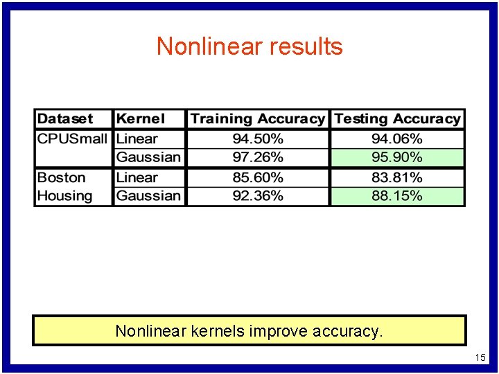
Nonlinear results Nonlinear kernels improve accuracy. 15

Focus 2: Support Vector Tolerant Regression

Regression Approach Summary l Quadratic Loss Function – Standard method in statistics – Over-emphasizes outliers l Linear Loss Function (1 -norm) – Formulates well as a linear program – Over-emphasizes small errors l Huber Loss Function (hybrid approach) – Appropriate emphasis on large and small errors 17

Optimization problem l Find w, b such that: l Bound the error by s: l Minimize the error: Minimize the magnitude of the error. 18

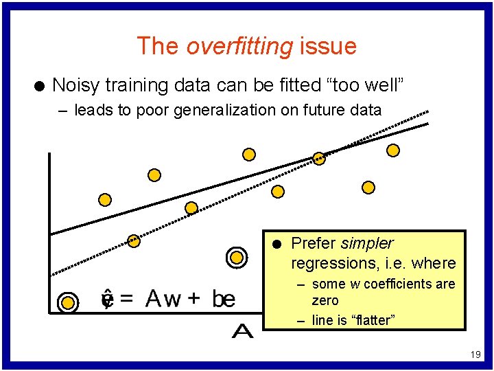
The overfitting issue l Noisy training data can be fitted “too well” – leads to poor generalization on future data l Prefer simpler regressions, i. e. where – some w coefficients are zero – line is “flatter” 19

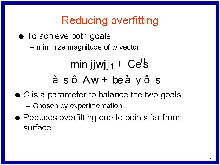
Reducing overfitting l To achieve both goals – minimize magnitude of w vector l C is a parameter to balance the two goals – Chosen by experimentation l Reduces overfitting due to points far from surface 20

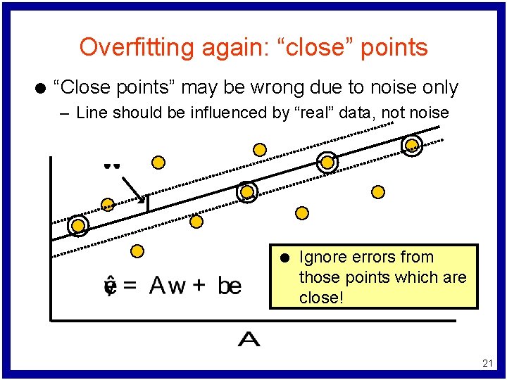
Overfitting again: “close” points l “Close points” may be wrong due to noise only – Line should be influenced by “real” data, not noise l Ignore errors from those points which are close! 21

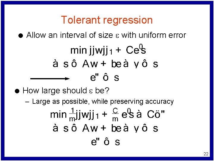
Tolerant regression l l Allow an interval of size e with uniform error How large should e be? – Large as possible, while preserving accuracy 22

How about a nonlinear surface? 23

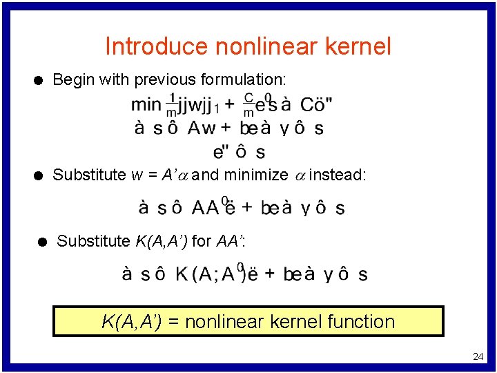
Introduce nonlinear kernel l Begin with previous formulation: l Substitute w = A’a and minimize a instead: l Substitute K(A, A’) for AA’: K(A, A’) = nonlinear kernel function 24

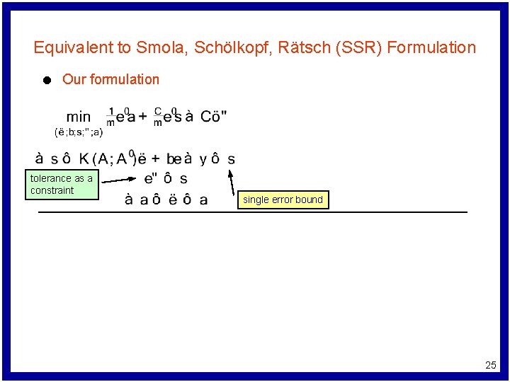
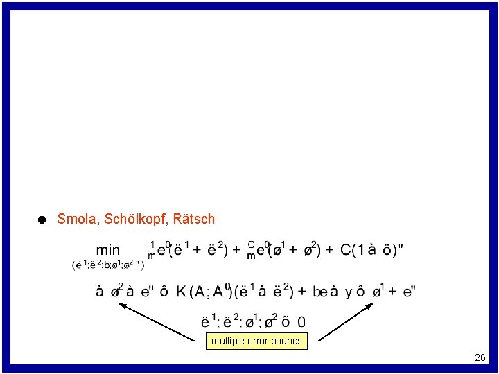
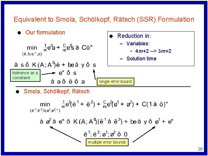
Equivalent to Smola, Schölkopf, Rätsch (SSR) Formulation l Our formulation tolerance as a constraint single error bound 25

l Smola, Schölkopf, Rätsch multiple error bounds 26

l Reduction in: – Variables: • 4 m+2 --> 3 m+2 – Solution time 27

Equivalent to Smola, Schölkopf, Rätsch (SSR) Formulation l Our formulation l Reduction in: – Variables: • 4 m+2 --> 3 m+2 – Solution time tolerance as a constraint l single error bound Smola, Schölkopf, Rätsch multiple error bounds 28

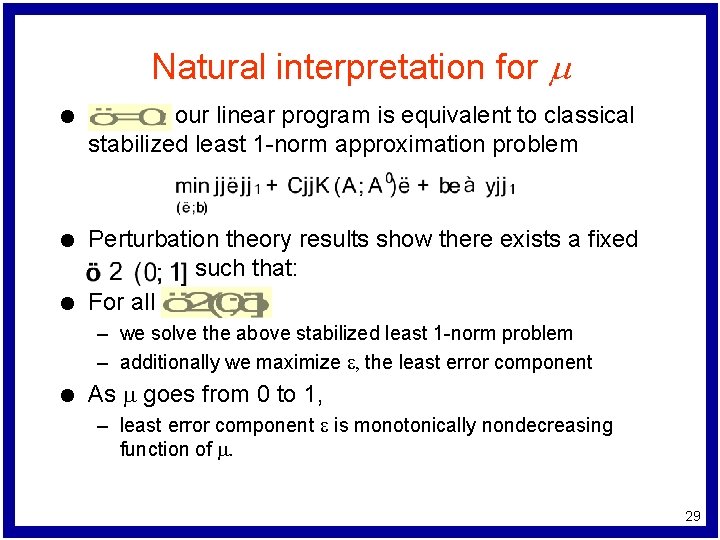
Natural interpretation for m l our linear program is equivalent to classical stabilized least 1 -norm approximation problem l Perturbation theory results show there exists a fixed such that: For all l – we solve the above stabilized least 1 -norm problem – additionally we maximize e, the least error component l As m goes from 0 to 1, – least error component e is monotonically nondecreasing function of m. 29

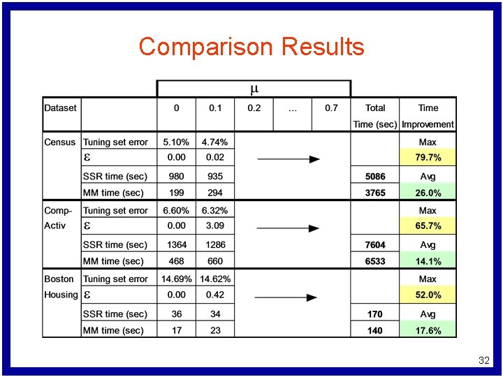
Numerical Testing l Two sets of tests – Compare computational times of our method (MM) and the SSR method – Row-column chunking for massive datasets l Datasets: – – l US Census Bureau Adult Dataset: 300, 000 points in R 11 Delve Comp-Activ Dataset: 8192 points in R 13 UCI Boston Housing Dataset: 506 points in R 13 Gaussian noise was added to each of these datasets. Hardware: Locop 2: Dell Power. Edge 6300 server with: – Four gigabytes of memory, 36 gigabytes of disk space – Windows NT Server 4. 0 – CPLEX 6. 5 solver 30

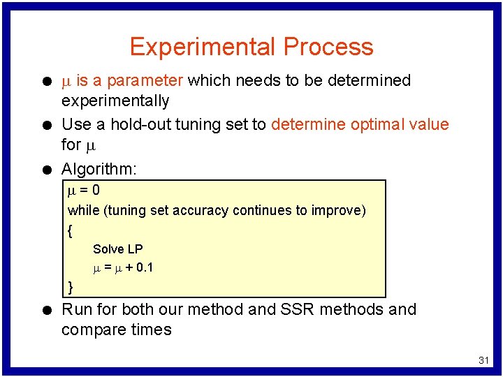
Experimental Process l l l m is a parameter which needs to be determined experimentally Use a hold-out tuning set to determine optimal value for m Algorithm: m=0 while (tuning set accuracy continues to improve) { Solve LP m = m + 0. 1 } l Run for both our method and SSR methods and compare times 31

Comparison Results 32

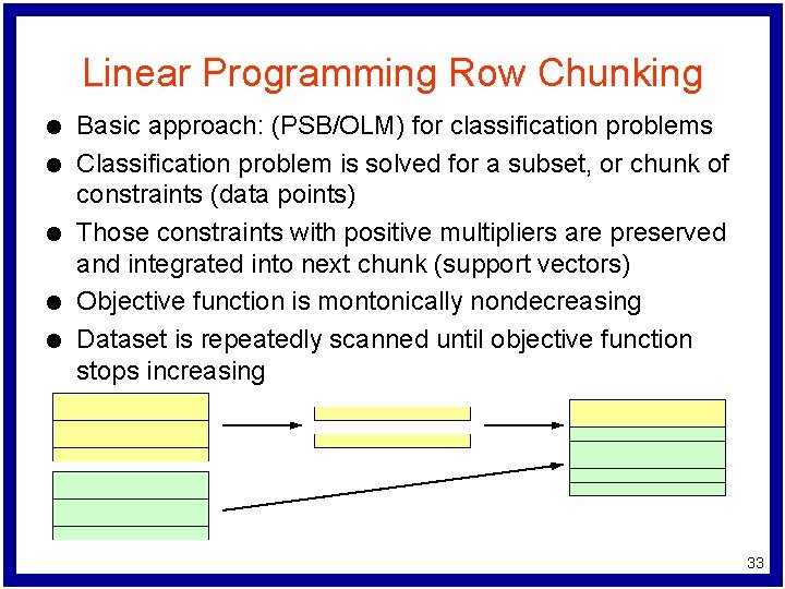
Linear Programming Row Chunking l l l Basic approach: (PSB/OLM) for classification problems Classification problem is solved for a subset, or chunk of constraints (data points) Those constraints with positive multipliers are preserved and integrated into next chunk (support vectors) Objective function is montonically nondecreasing Dataset is repeatedly scanned until objective function stops increasing 33

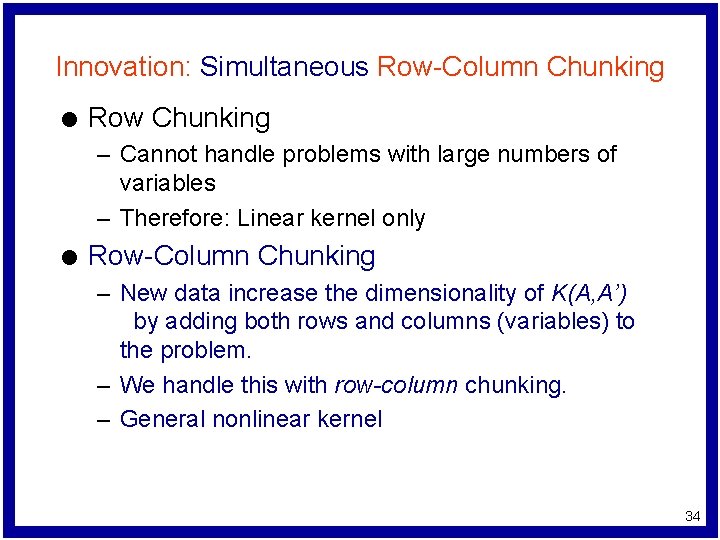
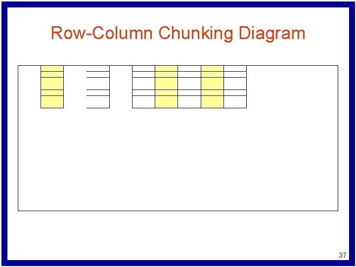
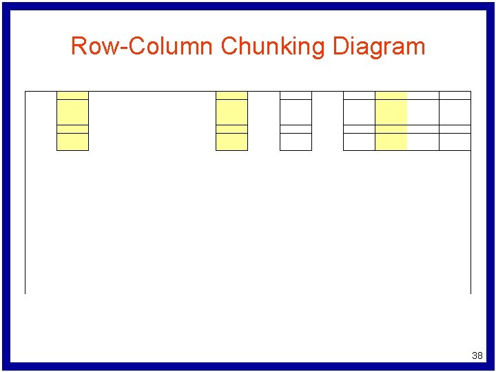
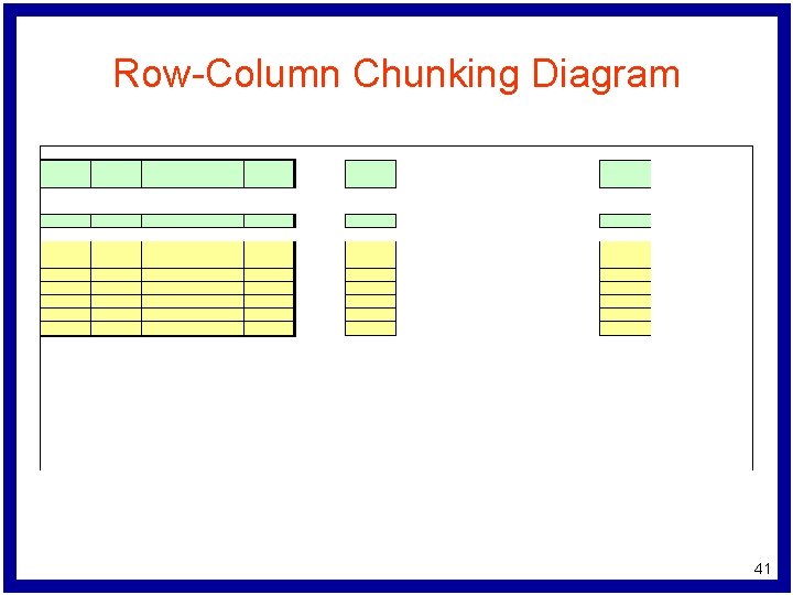
Innovation: Simultaneous Row-Column Chunking l Row Chunking – Cannot handle problems with large numbers of variables – Therefore: Linear kernel only l Row-Column Chunking – New data increase the dimensionality of K(A, A’) by adding both rows and columns (variables) to the problem. – We handle this with row-column chunking. – General nonlinear kernel 34

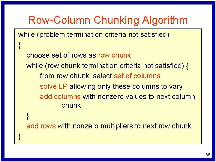
Row-Column Chunking Algorithm while (problem termination criteria not satisfied) { choose set of rows as row chunk while (row chunk termination criteria not satisfied) { from row chunk, select set of columns solve LP allowing only these columns to vary add columns with nonzero values to next column chunk } add rows with nonzero multipliers to next row chunk } 35

Row-Column Chunking Diagram 36

Row-Column Chunking Diagram 37

Row-Column Chunking Diagram 38

Row-Column Chunking Diagram 39

Row-Column Chunking Diagram 40

Row-Column Chunking Diagram 41

Row-Column Chunking Diagram 42

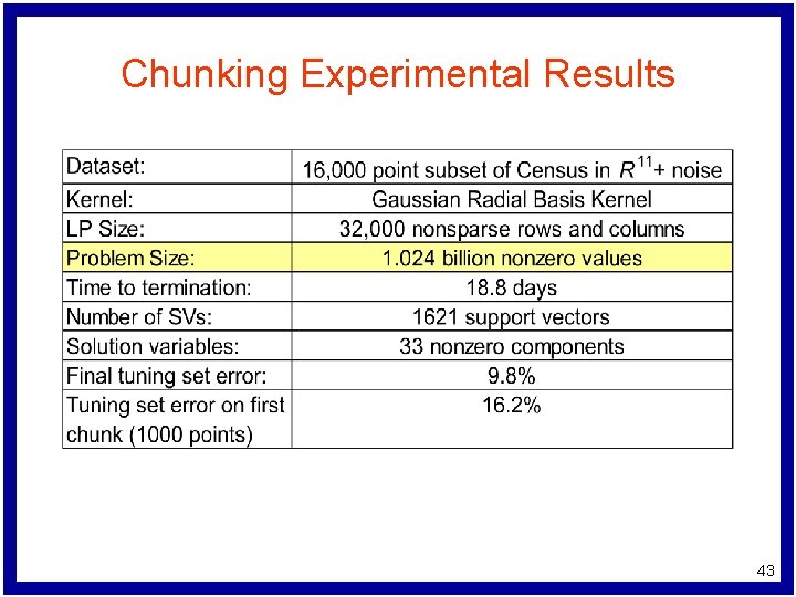
Chunking Experimental Results 43

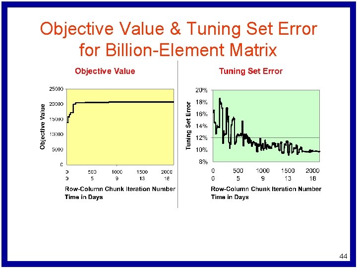
Objective Value & Tuning Set Error for Billion-Element Matrix 44

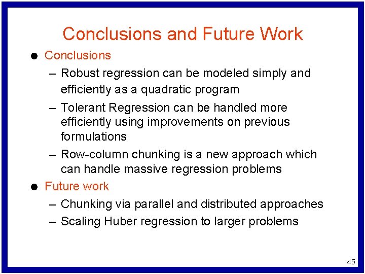
Conclusions and Future Work l l Conclusions – Robust regression can be modeled simply and efficiently as a quadratic program – Tolerant Regression can be handled more efficiently using improvements on previous formulations – Row-column chunking is a new approach which can handle massive regression problems Future work – Chunking via parallel and distributed approaches – Scaling Huber regression to larger problems 45

Questions? 46

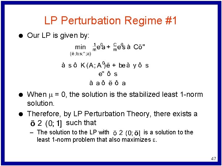
LP Perturbation Regime #1 l l l Our LP is given by: When m = 0, the solution is the stabilized least 1 -norm solution. Therefore, by LP Perturbation Theory, there exists a such that – The solution to the LP with is a solution to the least 1 -norm problem that also maximizes e. 47

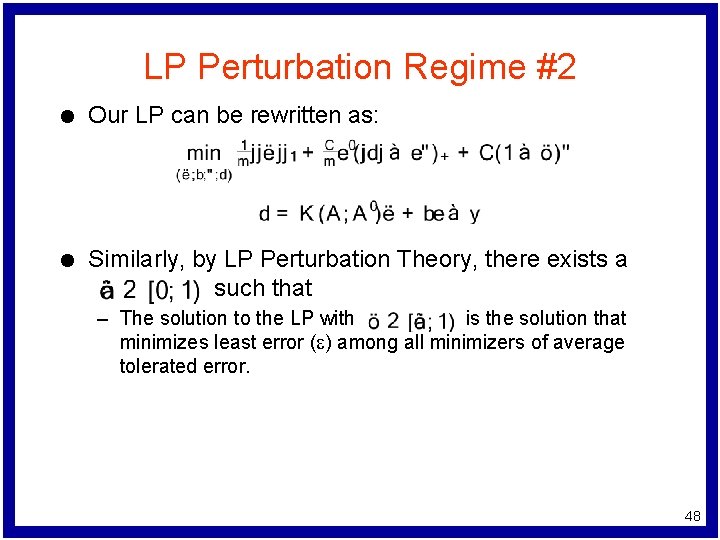
LP Perturbation Regime #2 l Our LP can be rewritten as: l Similarly, by LP Perturbation Theory, there exists a such that – The solution to the LP with is the solution that minimizes least error (e) among all minimizers of average tolerated error. 48

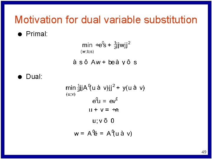
Motivation for dual variable substitution l Primal: l Dual: 49