Support Vector Machines SVM Xiyin Wu 2018 06

Support Vector Machines (SVM) Xiyin Wu 2018. 06. 14

SVM II. Multiclass SVM III. Conclusion

I. SVM

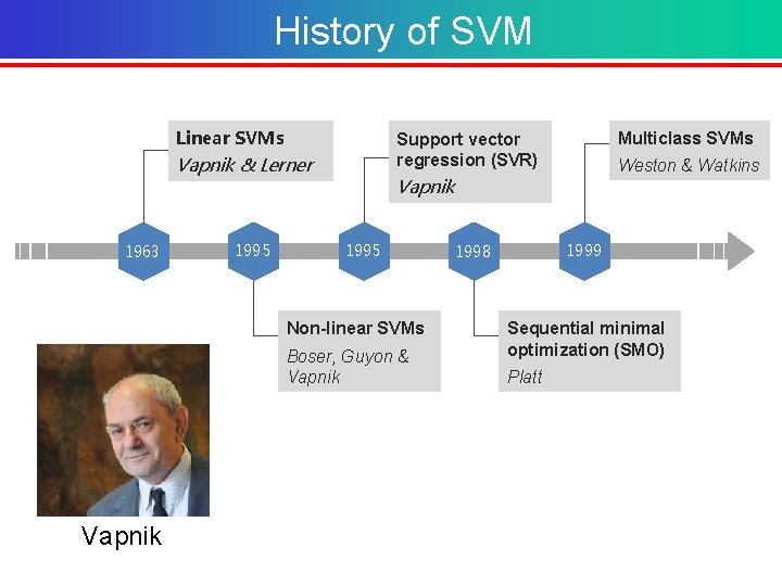
History of SVM Linear SVMs Vapnik & Lerner 1963 1995 Weston & Watkins Vapnik 1995 Non-linear SVMs Boser, Guyon & Vapnik Multiclass SVMs Support vector regression (SVR) 1999 1998 Sequential minimal optimization (SMO) Platt

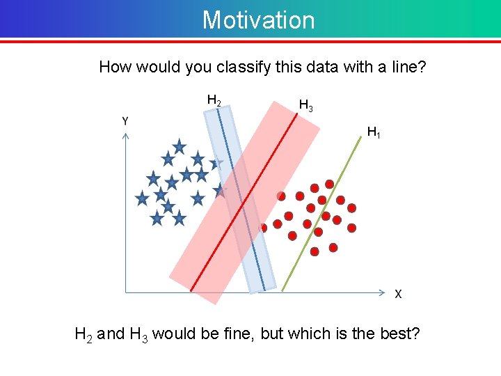
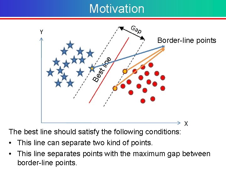
Motivation How would you classify this data with a line? H 2 H 3 H 1 H 2 and H 3 would be fine, but which is the best?

Motivation Be st lin e Border-line points The best line should satisfy the following conditions: • This line can separate two kind of points. • This line separates points with the maximum gap between border-line points.

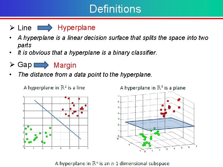
Definitions Ø Line Hyperplane • A hyperplane is a linear decision surface that splits the space into two parts • It is obvious that a hyperplane is a binary classifier. Ø Gap Margin • The distance from a data point to the hyperplane.

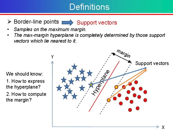
Definitions Ø Border-line points Support vectors • Samples on the maximum margin. • The max-margin hyperplane is completely determined by those support vectors which lie nearest to it. ma rgin Hy pe We should know: 1. How to express the hyperplane? 2. How to compute the margin? rpl an e Support vectors

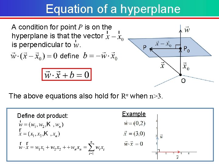
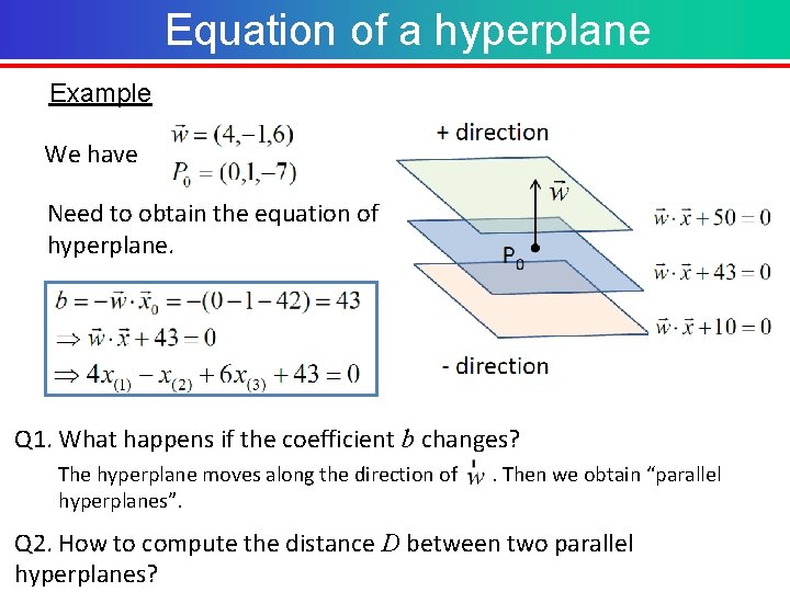
Equation of a hyperplane A condition for point P is on the hyperplane is that the vector is perpendicular to . The above equations also hold for Rn when n>3. Define dot product: Example

Equation of a hyperplane Example We have Need to obtain the equation of hyperplane. Q 1. What happens if the coefficient b changes? The hyperplane moves along the direction of . Then we obtain “parallel hyperplanes”. Q 2. How to compute the distance D between two parallel hyperplanes?

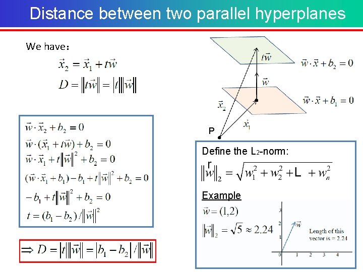
Distance between two parallel hyperplanes We have： P Define the L 2 -norm: Example

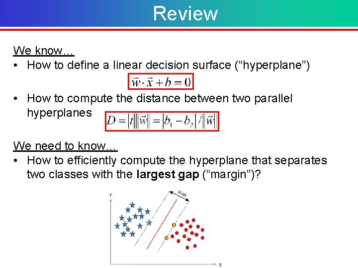
Review We know… • How to define a linear decision surface (“hyperplane”) • How to compute the distance between two parallel hyperplanes We need to know… • How to efficiently compute the hyperplane that separates two classes with the largest gap (“margin”)?

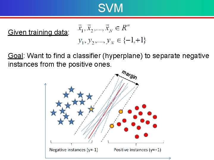
SVM Given training data: Goal: Want to find a classifier (hyperplane) to separate negative instances from the positive ones. ma rgin

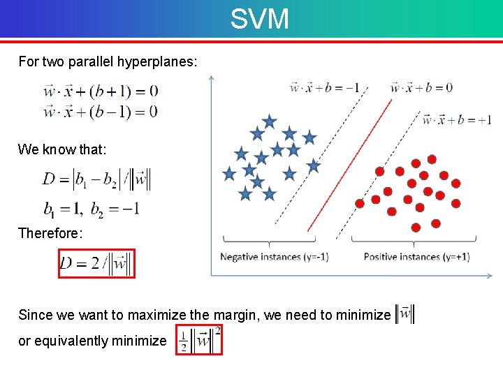
SVM For two parallel hyperplanes: We know that: Therefore: Since we want to maximize the margin, we need to minimize or equivalently minimize

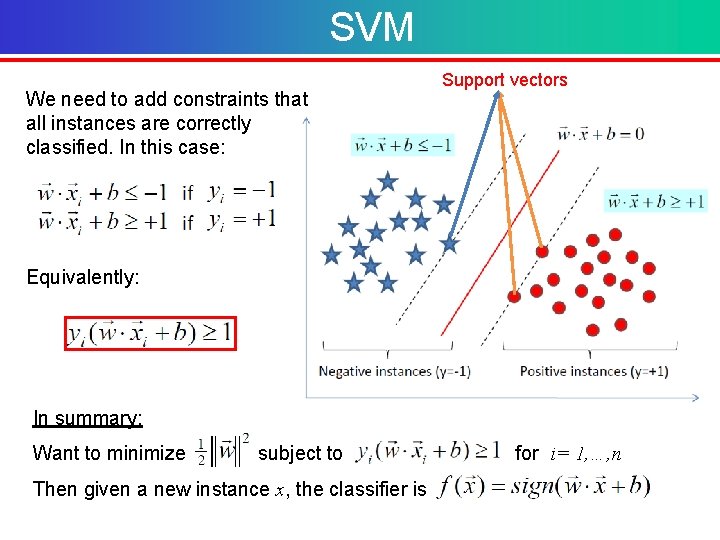
SVM We need to add constraints that all instances are correctly classified. In this case: Support vectors Equivalently: In summary: Want to minimize subject to for i= 1, …, n Then given a new instance x, the classifier is

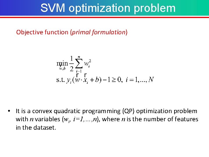
SVM optimization problem Objective function (primal formulation) • It is a convex quadratic programming (QP) optimization problem with n variables (wi, i=1, …, n), where n is the number of features in the dataset.

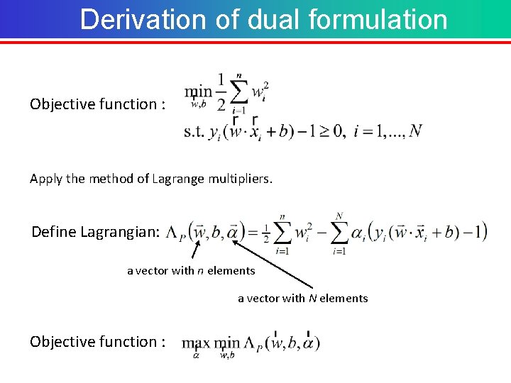
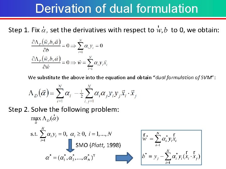
Derivation of dual formulation Objective function : Apply the method of Lagrange multipliers. Define Lagrangian: a vector with n elements a vector with N elements Objective function :

Derivation of dual formulation Step 1. Fix , set the derivatives with respect to 0, we obtain: We substitute the above into the equation and obtain “dual formulation of SVM”: Step 2. Solve the following problem: SMO (Platt, 1998)

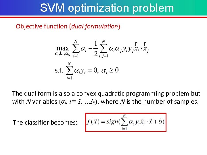
SVM optimization problem Objective function (dual formulation) The dual form is also a convex quadratic programming problem but with N variables (αi, i= 1, …, N), where N is the number of samples. The classifier becomes:

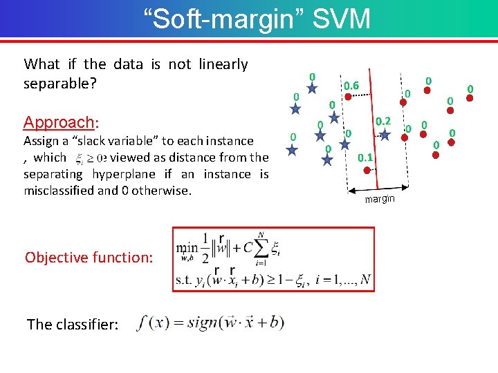
“Soft-margin” SVM What if the data is not linearly separable? Approach: Assign a “slack variable” to each instance , which can be viewed as distance from the separating hyperplane if an instance is misclassified and 0 otherwise. Objective function: The classifier: margin

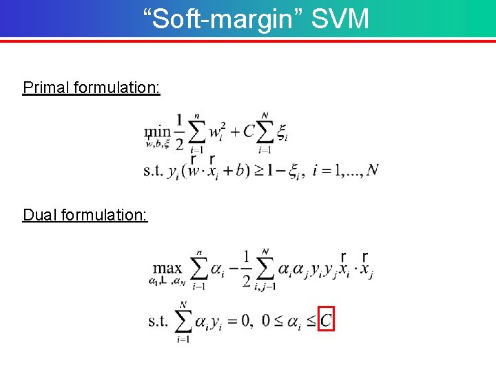
“Soft-margin” SVM Primal formulation: Dual formulation:

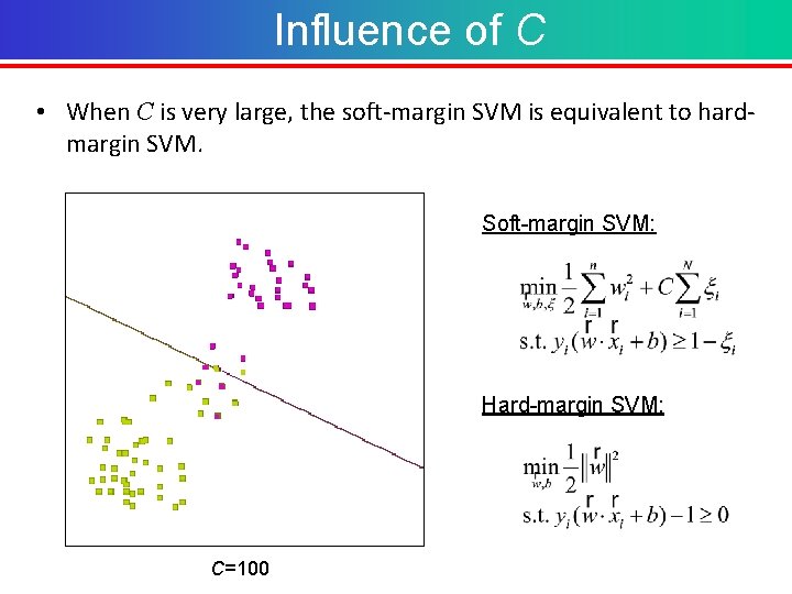
Influence of C • When C is very large, the soft-margin SVM is equivalent to hardmargin SVM. Soft-margin SVM: Hard-margin SVM: C=100

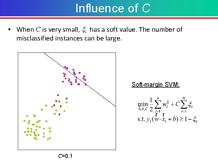
Influence of C • When C is very small, has a soft value. The number of misclassified instances can be large. Soft-margin SVM: C=0. 1

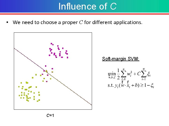
Influence of C • We need to choose a proper C for different applications. Soft-margin SVM: C=1

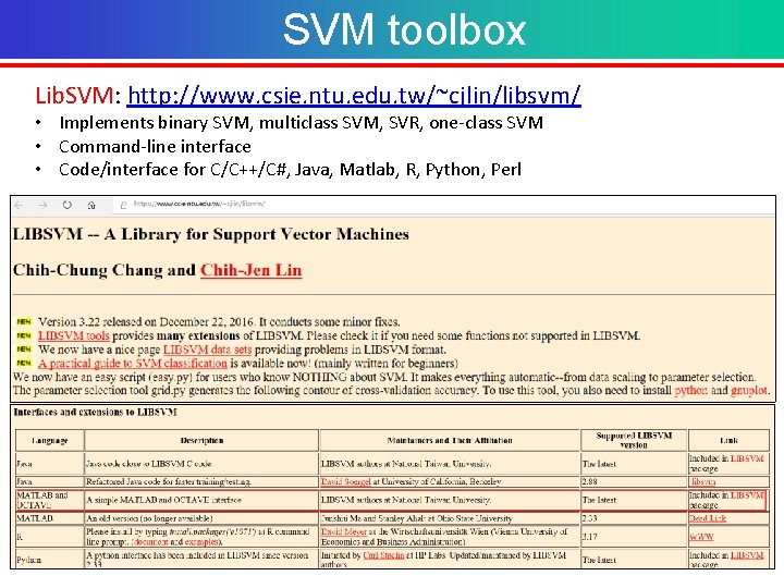
SVM toolbox Lib. SVM: http: //www. csie. ntu. edu. tw/~cjlin/libsvm/ • Implements binary SVM, multiclass SVM, SVR, one-class SVM • Command-line interface • Code/interface for C/C++/C#, Java, Matlab, R, Python, Perl

SVM toolbox Functions 1. Read data [label_vector, instance_matrix] = libsvmread(‘data. txt’); 2. Save data libsvmwrite(‘data. txt’, label_vector, instance_matrix); 3. Training model = libsvmtrain(train_label, train_instance [, 'options']); 4. Predict [predicted_label, accuracy] 　= libsvmpredict(test_label, test_instance, model [, 'options']); options: -s svm_type : set type of SVM (default 0) 0 -- C-SVC -t kernel_type : set type of kernel function (default 2) 0 -- linear: u'*v 2 -- radial basis function: exp(-gamma*|u-v|^2) -c cost : set the parameter C of C-SVC (default 1)

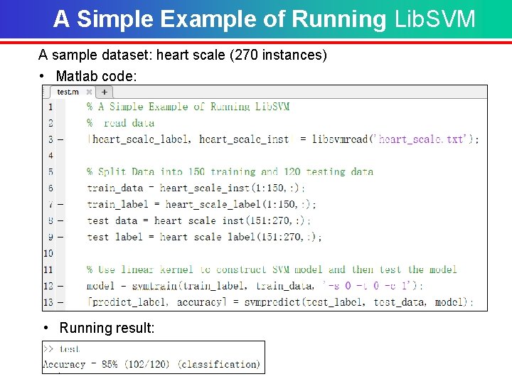
A Simple Example of Running Lib. SVM A sample dataset: heart scale (270 instances) • Matlab code: • Running result:

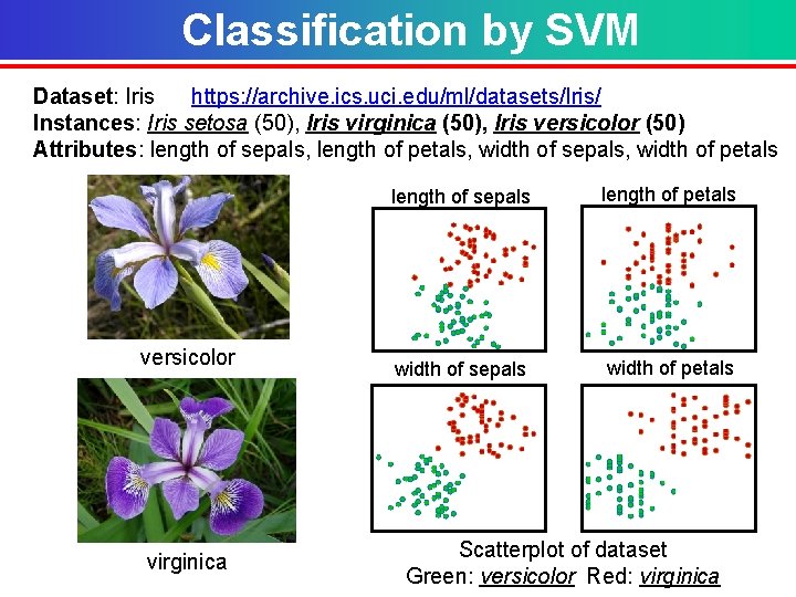
Classification by SVM Dataset: Iris https: //archive. ics. uci. edu/ml/datasets/Iris/ Instances: Iris setosa (50), Iris virginica (50), Iris versicolor (50) Attributes: length of sepals, length of petals, width of sepals, width of petals versicolor virginica length of sepals length of petals width of sepals width of petals Scatterplot of dataset Green: versicolor Red: virginica

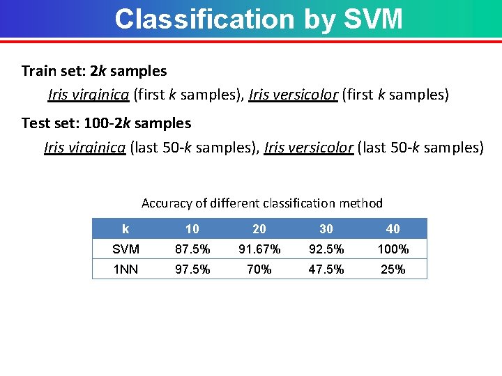
Classification by SVM Train set: 2 k samples Iris virginica (first k samples), Iris versicolor (first k samples) Test set: 100 -2 k samples Iris virginica (last 50 -k samples), Iris versicolor (last 50 -k samples) Accuracy of different classification method k 10 20 30 40 SVM 87. 5% 91. 67% 92. 5% 100% 1 NN 97. 5% 70% 47. 5% 25%

II. Multiclass SVM

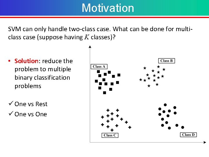
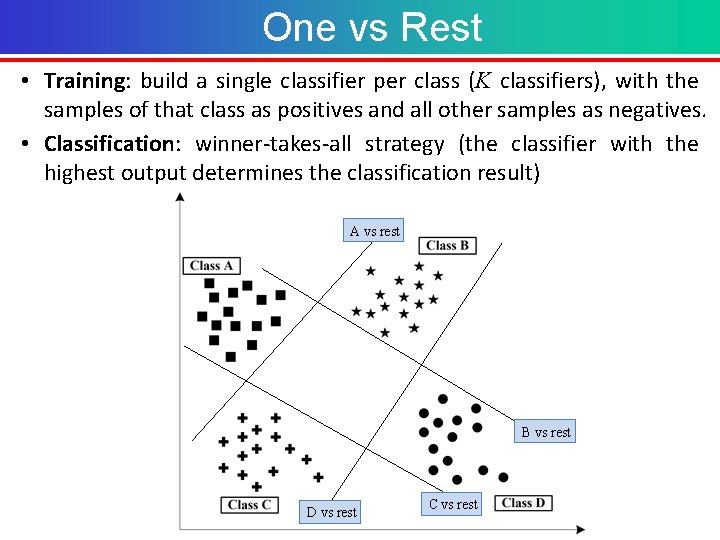
Motivation SVM can only handle two-class case. What can be done for multiclass case (suppose having K classes)? • Solution: reduce the problem to multiple binary classification problems ü One vs Rest ü One vs One

One vs Rest • Training: build a single classifier per class (K classifiers), with the samples of that class as positives and all other samples as negatives. • Classification: winner-takes-all strategy (the classifier with the highest output determines the classification result) A vs rest B vs rest D vs rest C vs rest

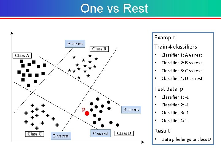
One vs Rest Example A vs rest Train 4 classifiers: • Classifier 1: A vs rest • Classifier 2: B vs rest • Classifier 3: C vs rest • Classifier 4: D vs rest Test data p p D vs rest B vs rest C vs rest • Classifier 1: -1 • Classifier 2: -1 • Classifier 3: -1 • Classifier 4: 1 Result • Data p belongs to class D

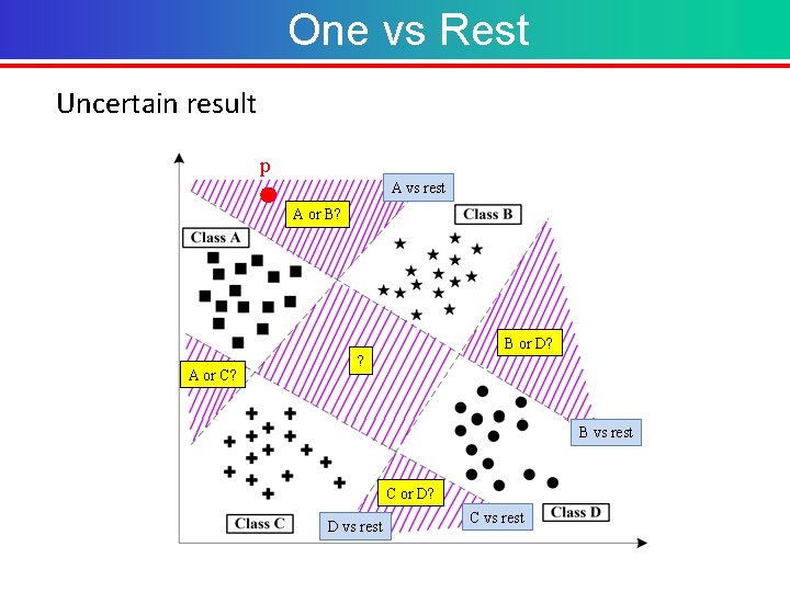
One vs Rest Uncertain result p A vs rest A or B? B or D? A or C? ? B vs rest C or D? D vs rest C vs rest

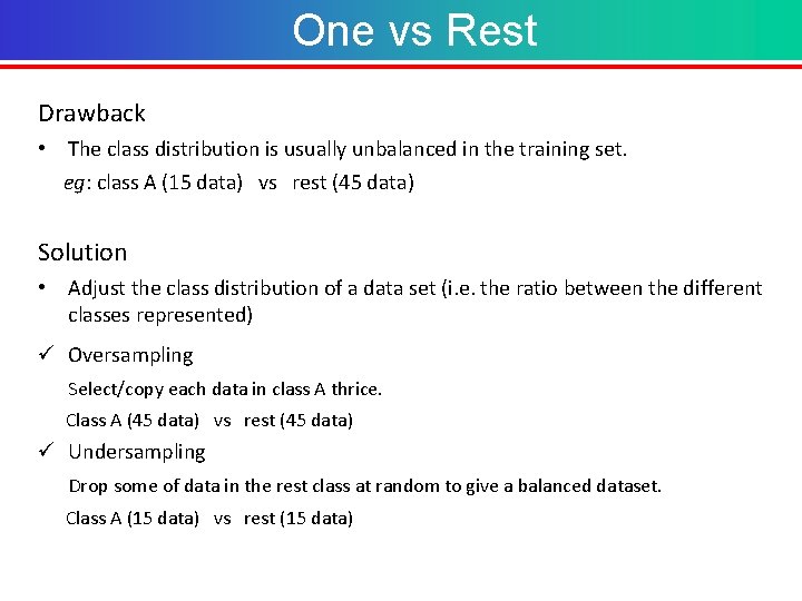
One vs Rest Drawback • The class distribution is usually unbalanced in the training set. eg: class A (15 data) vs rest (45 data) Solution • Adjust the class distribution of a data set (i. e. the ratio between the different classes represented) ü Oversampling Select/copy each data in class A thrice. Class A (45 data) vs rest (45 data) ü Undersampling Drop some of data in the rest class at random to give a balanced dataset. Class A (15 data) vs rest (15 data)

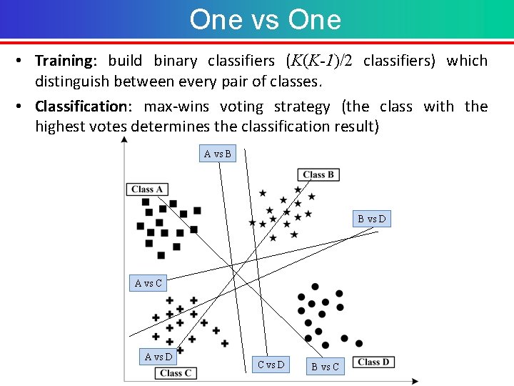
One vs One • Training: build binary classifiers (K(K-1)/2 classifiers) which distinguish between every pair of classes. • Classification: max-wins voting strategy (the class with the highest votes determines the classification result) A vs B B vs D A vs C A vs D C vs D B vs C

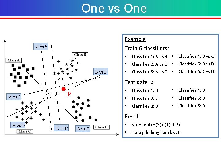
One vs One Example Train 6 classifiers: A vs B B vs D • Classifier 1: A vs B • Classifier 4: B vs C • Classifier 2: A vs C • Classifier 5: B vs D • Classifier 3: A vs D • Classifier 6: C vs D Test data p A vs C p • Classifier 1: B • Classifier 4: B • Classifier 2: C • Classifier 5: B • Classifier 3: D • Classifier 6: D Result A vs D C vs D B vs C • Vote: A(0) B(3) C(1) D(2) • Data p belongs to class B

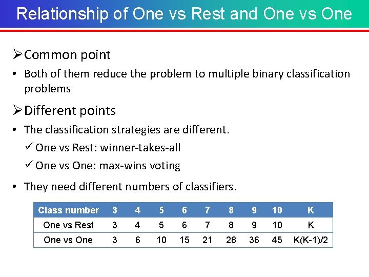
Relationship of One vs Rest and One vs One ØCommon point • Both of them reduce the problem to multiple binary classification problems ØDifferent points • The classification strategies are different. ü One vs Rest: winner-takes-all ü One vs One: max-wins voting • They need different numbers of classifiers. Class number 3 4 5 6 7 8 9 10 K One vs Rest 3 4 5 6 7 8 9 10 K One vs One 3 6 10 15 21 28 36 45 K(K-1)/2

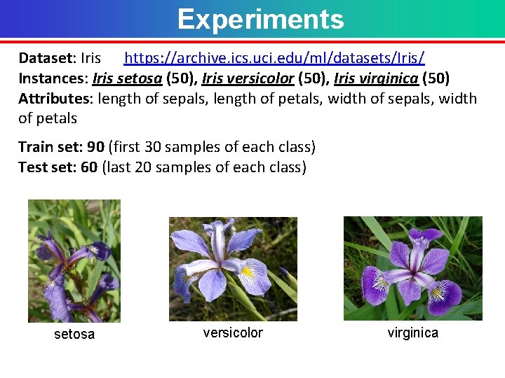
Experiments Dataset: Iris https: //archive. ics. uci. edu/ml/datasets/Iris/ Instances: Iris setosa (50), Iris versicolor (50), Iris virginica (50) Attributes: length of sepals, length of petals, width of sepals, width of petals Train set: 90 (first 30 samples of each class) Test set: 60 (last 20 samples of each class) setosa versicolor virginica

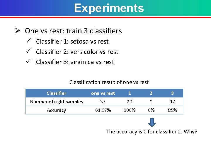
Experiments Ø One vs rest: train 3 classifiers ü Classifier 1: setosa vs rest ü Classifier 2: versicolor vs rest ü Classifier 3: virginica vs rest Classification result of one vs rest Classifier one vs rest 1 2 3 Number of right samples 37 20 0 17 Accuracy 61. 67% 100% 0% 85% The accuracy is 0 for classifier 2. Why?

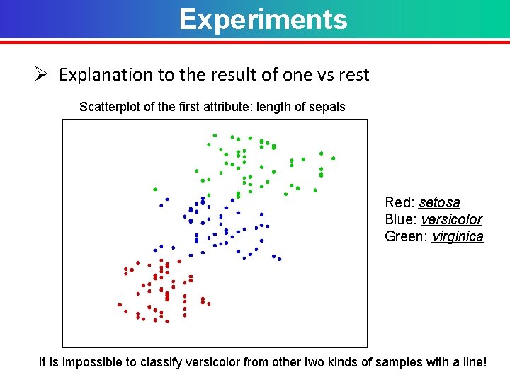
Experiments Ø Explanation to the result of one vs rest Scatterplot of the first attribute: length of sepals Red: setosa Blue: versicolor Green: virginica It is impossible to classify versicolor from other two kinds of samples with a line!

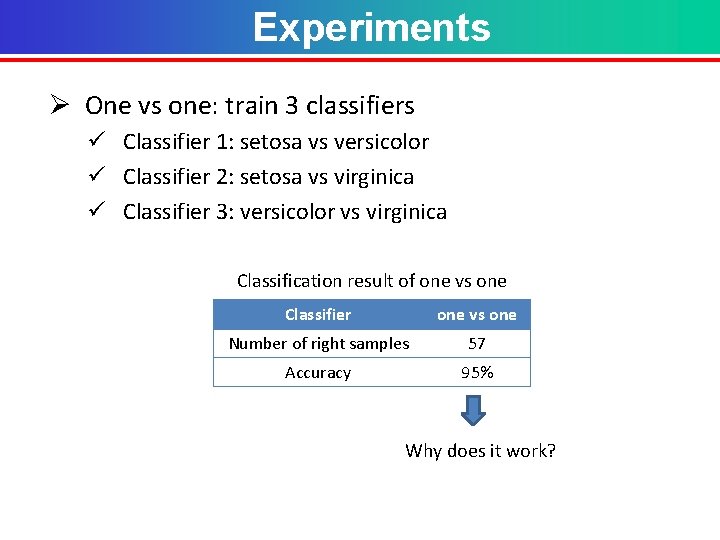
Experiments Ø One vs one: train 3 classifiers ü Classifier 1: setosa vs versicolor ü Classifier 2: setosa vs virginica ü Classifier 3: versicolor vs virginica Classification result of one vs one Classifier one vs one Number of right samples 57 Accuracy 95% Why does it work?

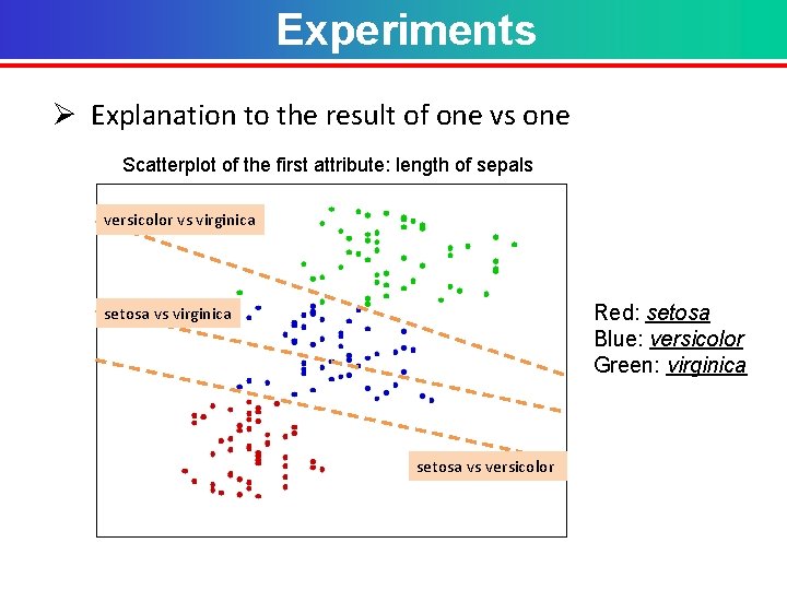
Experiments Ø Explanation to the result of one vs one Scatterplot of the first attribute: length of sepals versicolor vs virginica Red: setosa Blue: versicolor Green: virginica setosa vs versicolor

III. Conclusion

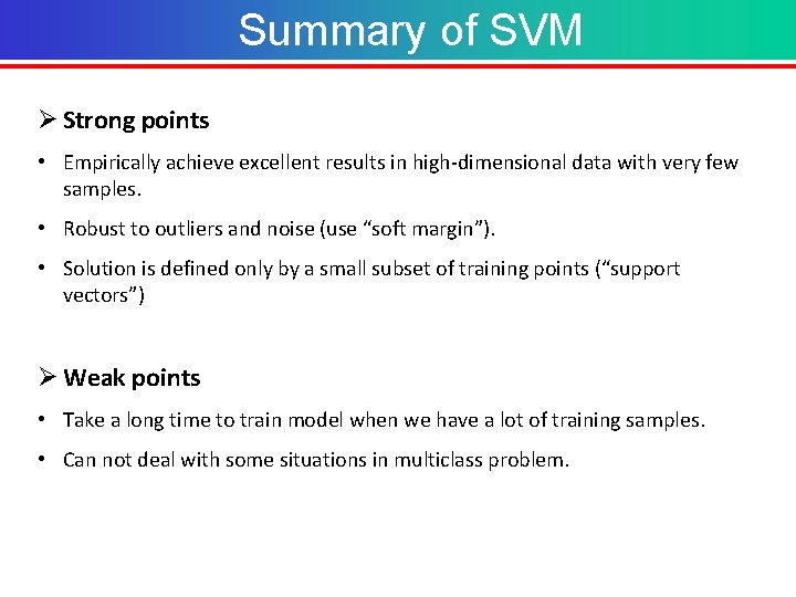
Summary of SVM Ø Strong points • Empirically achieve excellent results in high-dimensional data with very few samples. • Robust to outliers and noise (use “soft margin”). • Solution is defined only by a small subset of training points (“support vectors”) Ø Weak points • Take a long time to train model when we have a lot of training samples. • Can not deal with some situations in multiclass problem.

Bibliography • Boser BE, Guyon IM, Vapnik VN: A training algorithm for optimal margin classifiers. Proceedings of the Fifth Annual Workshop on Computational Learning Theory (COLT)1992: 144 -152. • Burges CJC: A tutorial on support vector machines for pattern recognition. Data Mining and Knowledge Discovery 1998, 2: 121 -167. • Schölkopf B, Burges CJC, Smola AJ: Advances in kernel methods: support vector learning. Cambridge, Mass: MIT Press; 1999. • Vapnik VN: Statistical learning theory. New York: Wiley; 1998. • Platt JC, Cristianini N, Shawe-Taylor J: Large margin DAGs for multiclassification. Advances in Neural Information Processing Systems (NIPS)2000, 12: 547 -553. • Smola. A J, Schölkopf B: A tutorial on support vector regression. Statistics and Computing 2004, 14: 199 -222. • Hur BA, Horn D, Siegelmann HT, Vapnik V: Support vector clustering. Journal of Machine Learning Research 2001, 2: 125– 137. • Guyon I, Elisseeff A: An introduction to variable and feature selection. Journal of Machine Learning Research 2003, 3: 1157 -1182.

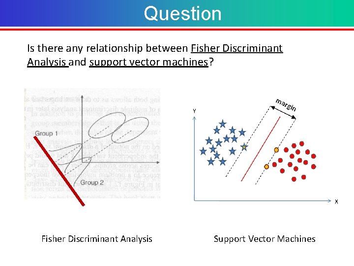
Question Is there any relationship between Fisher Discriminant Analysis and support vector machines? ma Fisher Discriminant Analysis rgin Support Vector Machines

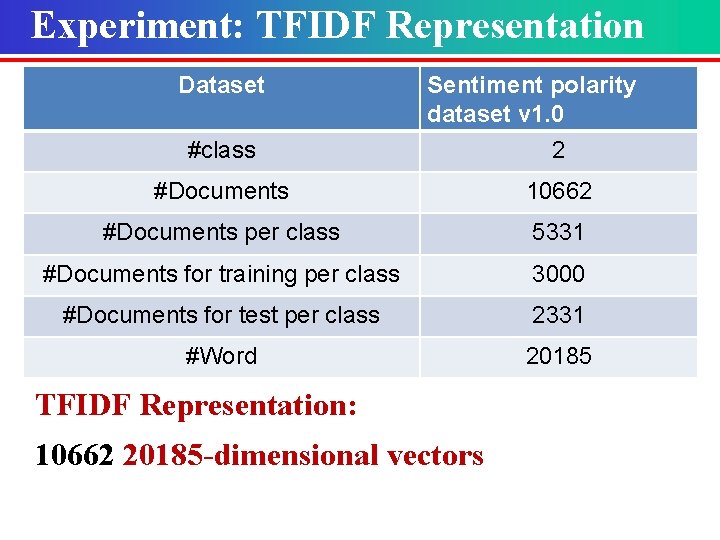
Experiment: TFIDF Representation Dataset #class Sentiment polarity dataset v 1. 0 2 #Documents 10662 #Documents per class 5331 #Documents for training per class 3000 #Documents for test per class 2331 #Word 20185 TFIDF Representation: 10662 20185 -dimensional vectors

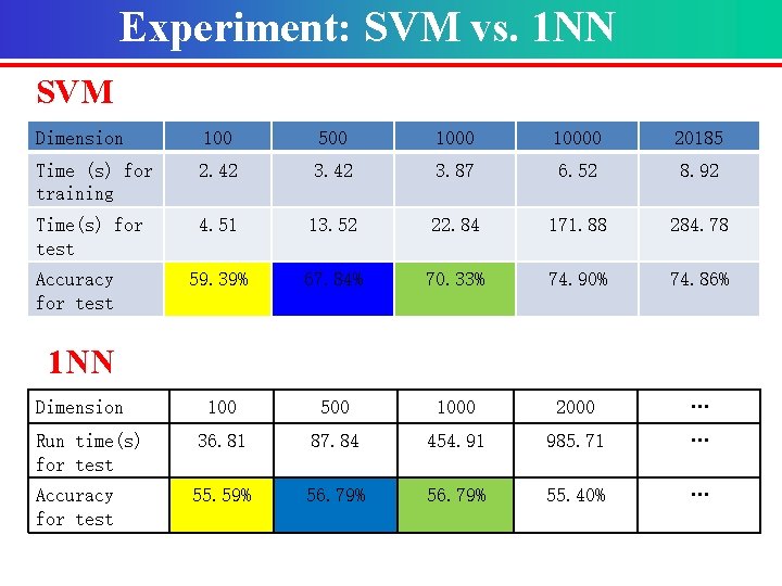
Experiment: SVM vs. 1 NN SVM Dimension 100 500 10000 20185 Time (s) for training 2. 42 3. 87 6. 52 8. 92 Time(s) for test 4. 51 13. 52 22. 84 171. 88 284. 78 59. 39% 67. 84% 70. 33% 74. 90% 74. 86% 100 500 1000 2000 … Run time(s) for test 36. 81 87. 84 454. 91 985. 71 … Accuracy for test 55. 59% 56. 79% 55. 40% … Accuracy for test 1 NN Dimension

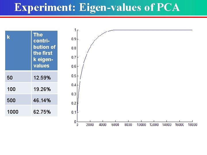
Experiment: Eigen-values of PCA k The contribution of the first k eigenvalues 50 12. 59% 100 19. 26% 500 46. 14% 1000 62. 75%

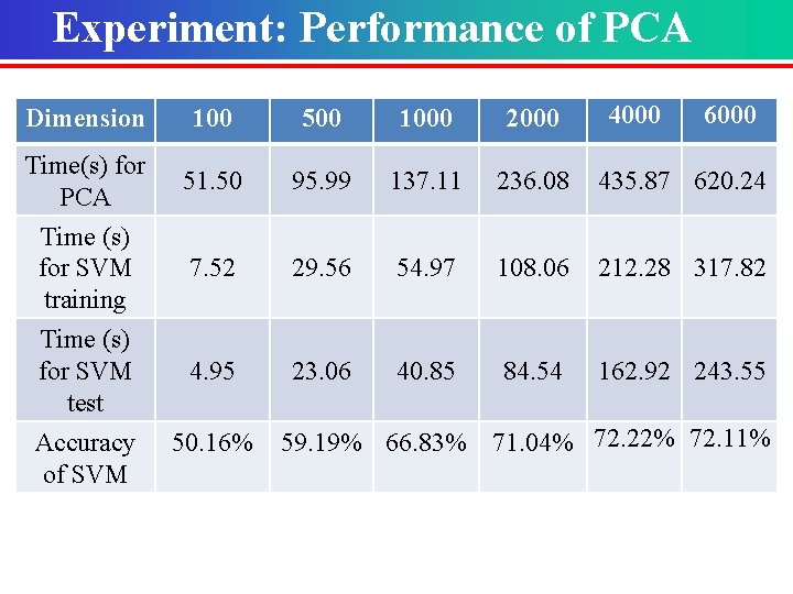
Experiment: Performance of PCA 4000 6000 Dimension 100 500 1000 2000 Time(s) for PCA 51. 50 95. 99 137. 11 236. 08 435. 87 620. 24 Time (s) for SVM training 7. 52 29. 56 54. 97 108. 06 212. 28 317. 82 Time (s) for SVM test 4. 95 23. 06 40. 85 84. 54 162. 92 243. 55 Accuracy of SVM 50. 16% 59. 19% 66. 83% 71. 04% 72. 22% 72. 11%

Exercise Do an exercise on a sentiment dataset just following the experiment on page 48 -51 or Do an exercise on an image dataset just following the experiment on page 49 -51.

Thank you！ Xiyin Wu 2018. 06. 14