Support Vector Machines Note to other teachers and

Support Vector Machines Note to other teachers and users of these slides. Andrew would be delighted if you found this source material useful in giving your own lectures. Feel free to use these slides verbatim, or to modify them to fit your own needs. Power. Point originals are available. If you make use of a significant portion of these slides in your own lecture, please include this message, or the following link to the source repository of Andrew’s tutorials: http: //www. cs. cmu. edu/~awm/tutorials. Comments and corrections gratefully received. Andrew W. Moore Professor School of Computer Science Carnegie Mellon University www. cs. cmu. edu/~awm awm@cs. cmu. edu 412 -268 -7599 Copyright © 2001, 2003, Andrew W. Moore Nov 23 rd, 2001

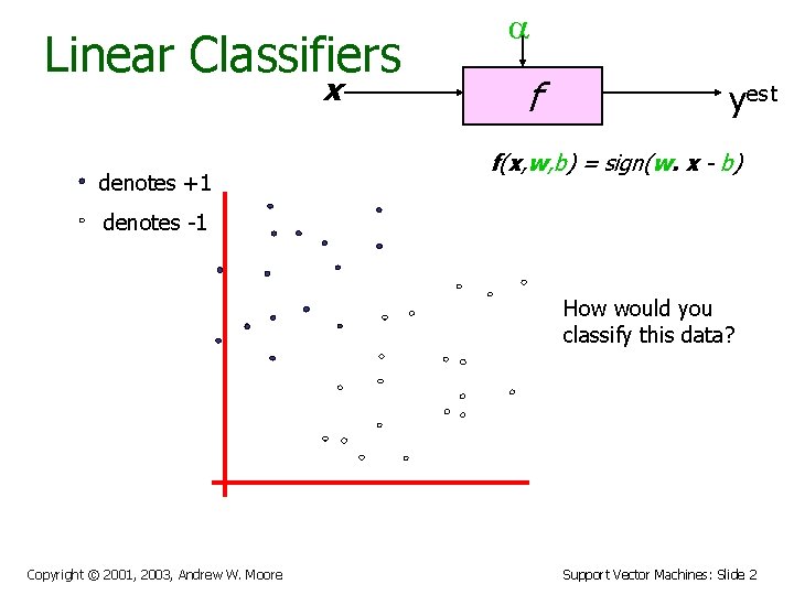
Linear Classifiers x denotes +1 a f yest f(x, w, b) = sign(w. x - b) denotes -1 How would you classify this data? Copyright © 2001, 2003, Andrew W. Moore Support Vector Machines: Slide 2

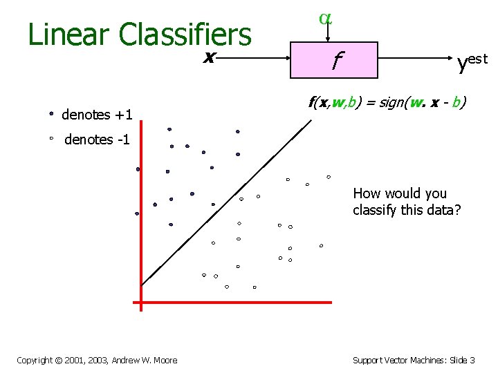
Linear Classifiers x denotes +1 a f yest f(x, w, b) = sign(w. x - b) denotes -1 How would you classify this data? Copyright © 2001, 2003, Andrew W. Moore Support Vector Machines: Slide 3

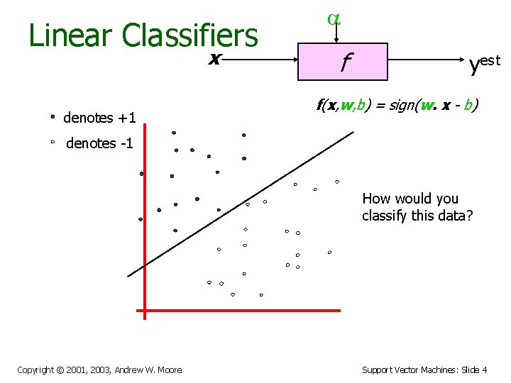
Linear Classifiers x denotes +1 a f yest f(x, w, b) = sign(w. x - b) denotes -1 How would you classify this data? Copyright © 2001, 2003, Andrew W. Moore Support Vector Machines: Slide 4

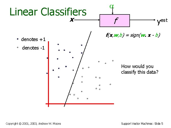
Linear Classifiers x denotes +1 a f yest f(x, w, b) = sign(w. x - b) denotes -1 How would you classify this data? Copyright © 2001, 2003, Andrew W. Moore Support Vector Machines: Slide 5

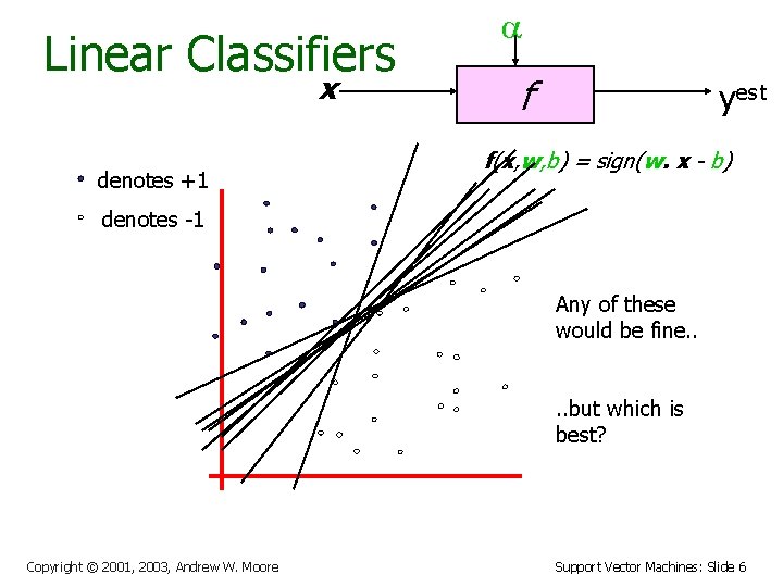
Linear Classifiers x denotes +1 a f yest f(x, w, b) = sign(w. x - b) denotes -1 Any of these would be fine. . but which is best? Copyright © 2001, 2003, Andrew W. Moore Support Vector Machines: Slide 6

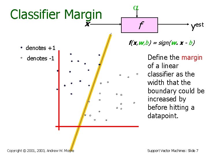
Classifier Margin x denotes +1 denotes -1 Copyright © 2001, 2003, Andrew W. Moore a f yest f(x, w, b) = sign(w. x - b) Define the margin of a linear classifier as the width that the boundary could be increased by before hitting a datapoint. Support Vector Machines: Slide 7

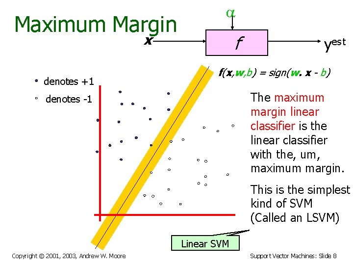
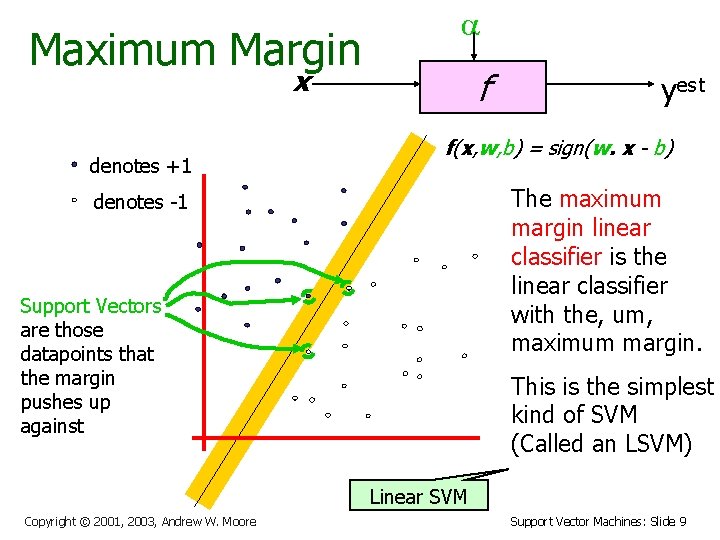
Maximum Margin a x denotes +1 f yest f(x, w, b) = sign(w. x - b) The maximum margin linear classifier is the linear classifier with the, um, maximum margin. denotes -1 This is the simplest kind of SVM (Called an LSVM) Linear SVM Copyright © 2001, 2003, Andrew W. Moore Support Vector Machines: Slide 8

Maximum Margin a x denotes +1 f yest f(x, w, b) = sign(w. x - b) The maximum margin linear classifier is the linear classifier with the, um, maximum margin. denotes -1 Support Vectors are those datapoints that the margin pushes up against This is the simplest kind of SVM (Called an LSVM) Linear SVM Copyright © 2001, 2003, Andrew W. Moore Support Vector Machines: Slide 9

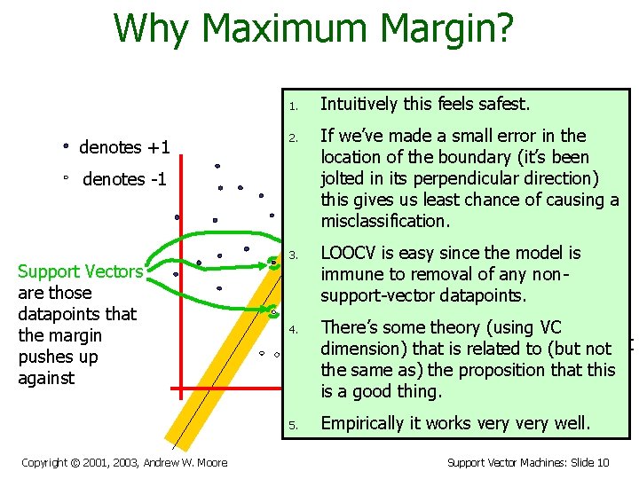
Why Maximum Margin? 1. denotes +1 2. denotes -1 Support Vectors are those datapoints that the margin pushes up against 3. f(x, w, b) = sign(w. - b) If we’ve made a small error inxthe location of the boundary (it’s been The maximum jolted in its perpendicular direction) this gives us leastmargin chance linear of causing a misclassification. classifier is the LOOCV is easy since the classifier model is linear immune to removal of any with the, nonum, support-vector datapoints. maximum margin. 4. 5. Copyright © 2001, 2003, Andrew W. Moore Intuitively this feels safest. There’s some theory (using VC is the simplest dimension) that is. This related to (but not of SVM the same as) thekind proposition that this is a good thing. (Called an LSVM) Empirically it works very well. Support Vector Machines: Slide 10

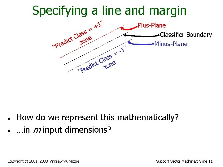
Specifying a line and margin ” 1 + = ss a l t C one c i z ed r P “ Plus-Plane Classifier Boundary 1” = Minus-Plane ss a l t C one c i z red “P • • How do we represent this mathematically? …in m input dimensions? Copyright © 2001, 2003, Andrew W. Moore Support Vector Machines: Slide 11

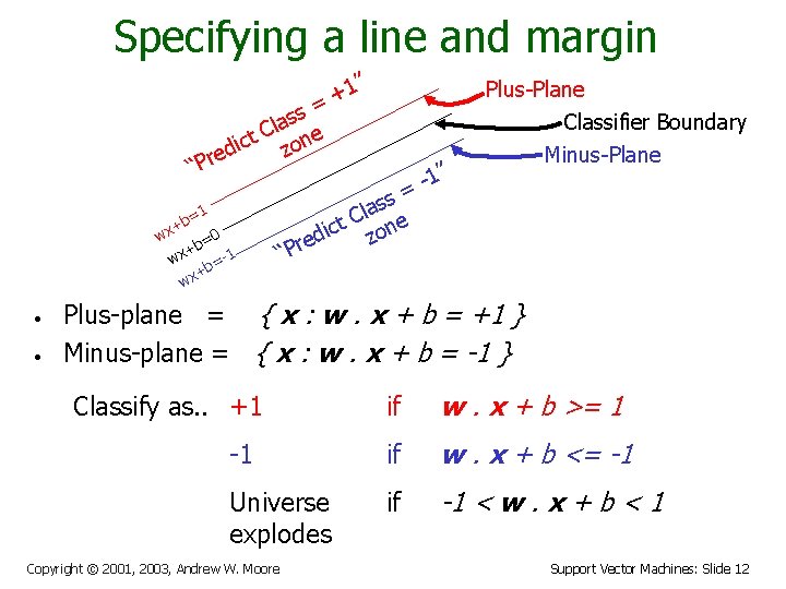
Specifying a line and margin ” 1 + = Plus-Plane Classifier Boundary ss a l t C one c i z ed r P “ =1 b + 0 wx b= + wx b=-1 + wx • • 1” = Minus-Plane ss a l t C one c i z red “P Plus-plane = { x : w. x + b = +1 } Minus-plane = { x : w. x + b = -1 } if w. x + b >= 1 -1 if w. x + b <= -1 Universe explodes if -1 < w. x + b < 1 Classify as. . +1 Copyright © 2001, 2003, Andrew W. Moore Support Vector Machines: Slide 12

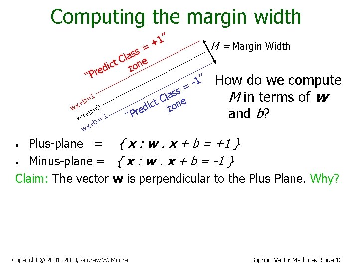
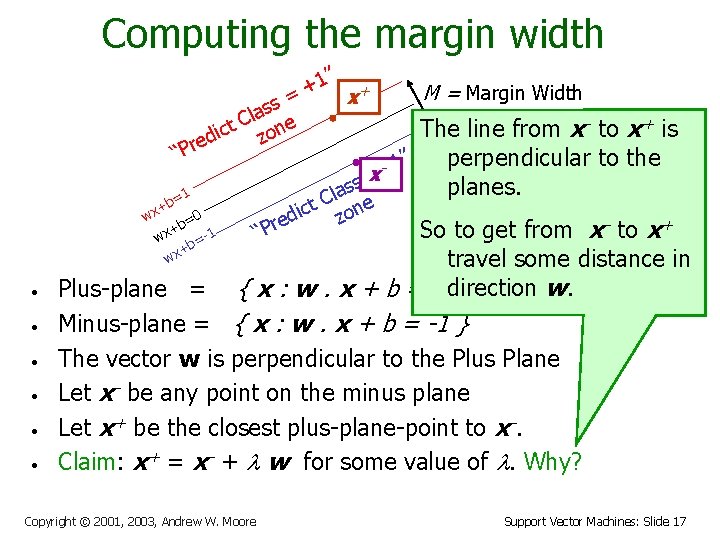
Computing the margin width ” 1 + = ss a l t C one c i z ed r P “ =1 b + 0 wx b= + wx b=-1 + wx M = Margin Width 1” = “P ss a l t C one c i z red How do we compute M in terms of w and b? Plus-plane = { x : w. x + b = +1 } • Minus-plane = { x : w. x + b = -1 } Claim: The vector w is perpendicular to the Plus Plane. Why? • Copyright © 2001, 2003, Andrew W. Moore Support Vector Machines: Slide 13

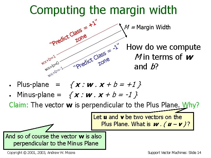
Computing the margin width ” 1 + = ss a l t C one c i z ed r P “ =1 b + 0 wx b= + wx b=-1 + wx M = Margin Width 1” = ss a l t C one c i z red “P How do we compute M in terms of w and b? Plus-plane = { x : w. x + b = +1 } • Minus-plane = { x : w. x + b = -1 } Claim: The vector w is perpendicular to the Plus Plane. Why? • Let u and v be two vectors on the Plus Plane. What is w. ( u – v ) ? And so of course the vector w is also perpendicular to the Minus Plane Copyright © 2001, 2003, Andrew W. Moore Support Vector Machines: Slide 14

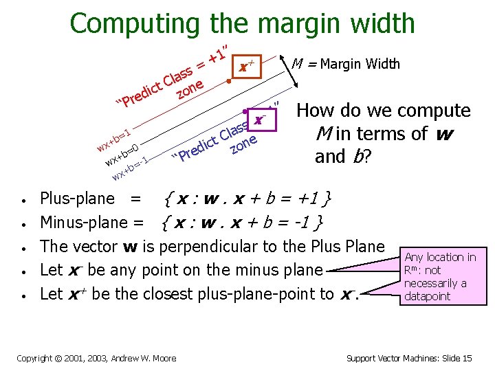
Computing the margin width 1” + + M = Margin Width = x s s la e C ct zon i d e “Pr 1” How do we compute x = s s la M in terms of w =1 C b e t + wx dic zon =0 e b r + and b? “P -1 wx = +b x w • • • Plus-plane = { x : w. x + b = +1 } Minus-plane = { x : w. x + b = -1 } The vector w is perpendicular to the Plus Plane Let x- be any point on the minus plane Let x+ be the closest plus-plane-point to x-. Copyright © 2001, 2003, Andrew W. Moore Any location in mm: : not R necessarily a datapoint Support Vector Machines: Slide 15

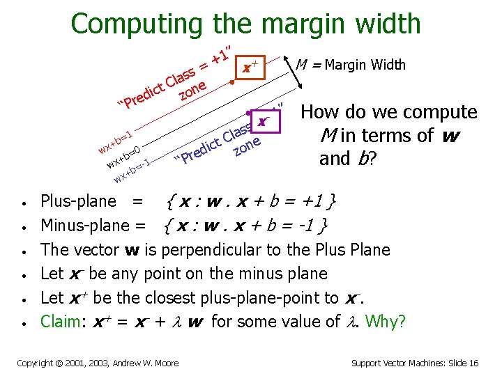
Computing the margin width 1” + + M = Margin Width = x s s la e C ct zon i d e “Pr 1” How do we compute x = s s la M in terms of w =1 C b e t + wx dic zon =0 e b r + and b? “P -1 wx = +b x w • • • Plus-plane = { x : w. x + b = +1 } Minus-plane = { x : w. x + b = -1 } The vector w is perpendicular to the Plus Plane Let x- be any point on the minus plane Let x+ be the closest plus-plane-point to x-. Claim: x+ = x- + l w for some value of l. Why? Copyright © 2001, 2003, Andrew W. Moore Support Vector Machines: Slide 16

Computing the margin width 1” + + M = Margin Width = x s s la e C - to x+ is t n c The line from x i o z ed r P “ perpendicular to the do we compute 1” How x = s s planes. a 1 l M in terms of w = C b e t + wx dic zon =0 e b - to x+ r + P and b ? So to get from x 1 “ wx = wx • • • +b travel some distance in direction w. { x : w. x + b = +1 } Plus-plane = Minus-plane = { x : w. x + b = -1 } The vector w is perpendicular to the Plus Plane Let x- be any point on the minus plane Let x+ be the closest plus-plane-point to x-. Claim: x+ = x- + l w for some value of l. Why? Copyright © 2001, 2003, Andrew W. Moore Support Vector Machines: Slide 17

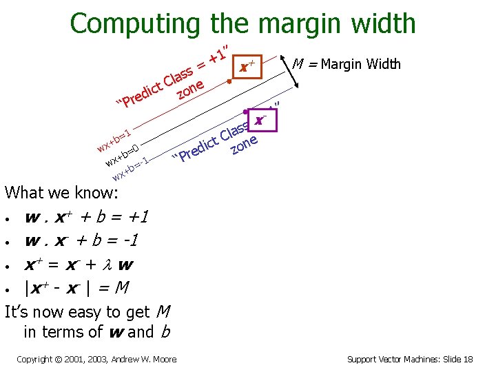
Computing the margin width 1” + + M = Margin Width = x s s la e C ct zon i d e “Pr 1” x = s s la =1 C b e t + c n i 0 o wx d z = re +b -1 P x “ w = +b x w What we know: • • w. x+ + b = +1 w. x- + b = -1 x+ = x- + l w |x + - x - | = M It’s now easy to get M in terms of w and b Copyright © 2001, 2003, Andrew W. Moore Support Vector Machines: Slide 18

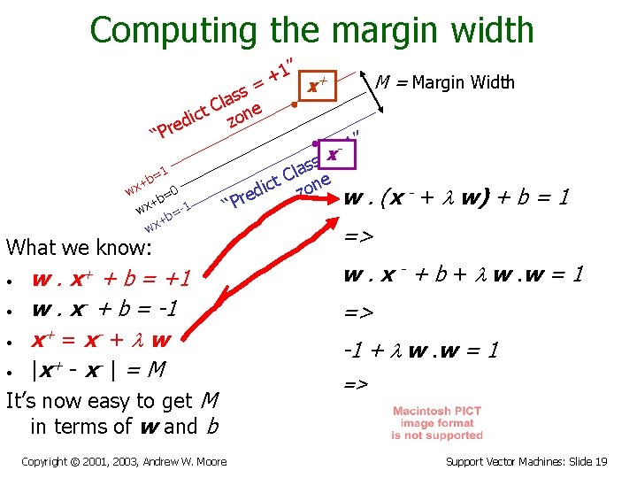
Computing the margin width 1” + + M = Margin Width = x s s la e C ct zon i d e “Pr 1” x = s s la =1 C b e t + c n i 0 o wx d - + l w) + b z = re w. (x +b -1 P x “ w = +b x w What we know: • • w. x+ + b = +1 w. x- + b = -1 x+ = x- + l w |x + - x - | = M It’s now easy to get M in terms of w and b Copyright © 2001, 2003, Andrew W. Moore =1 => w. x - + b + l w. w = 1 => -1 + l w. w = 1 => Support Vector Machines: Slide 19

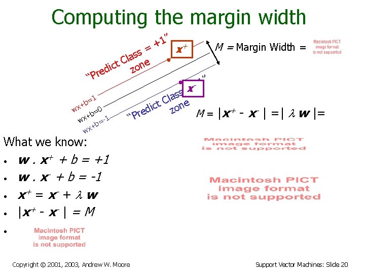
Computing the margin width 1” + + M = Margin Width = = x s s la e C ct zon i d e “Pr 1” x = s s la =1 C b e t + c n i 0 o wx d z = re M = |x+ - x- | =| l w |= +b -1 P x “ w = +b x w What we know: • • w. x+ + b = +1 w. x- + b = -1 x+ = x- + l w |x + - x - | = M • Copyright © 2001, 2003, Andrew W. Moore Support Vector Machines: Slide 20

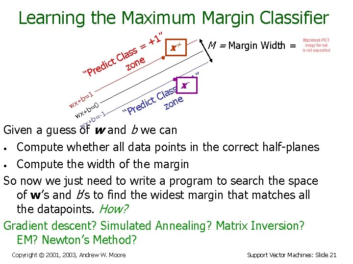
Learning the Maximum Margin Classifier 1” + + M = Margin Width = = x s s la e C ct zon i d e “Pr 1” x = s s la =1 C b e t + c n i 0 o wx d z = re +b -1 P x “ w = +b x w Given a guess of w and b we can • Compute whether all data points in the correct half-planes • Compute the width of the margin So now we just need to write a program to search the space of w’s and b’s to find the widest margin that matches all the datapoints. How? Gradient descent? Simulated Annealing? Matrix Inversion? EM? Newton’s Method? Copyright © 2001, 2003, Andrew W. Moore Support Vector Machines: Slide 21

Learning via Quadratic Programming • QP is a well-studied class of optimization algorithms to maximize a quadratic function of some real-valued variables subject to linear constraints. Copyright © 2001, 2003, Andrew W. Moore Support Vector Machines: Slide 22

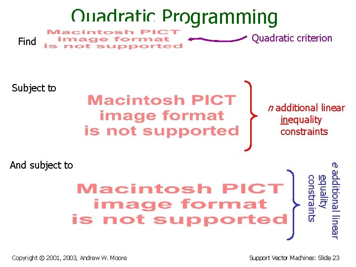
Quadratic Programming Find Quadratic criterion Subject to n additional linear inequality constraints Copyright © 2001, 2003, Andrew W. Moore e additional linear equality constraints And subject to Support Vector Machines: Slide 23

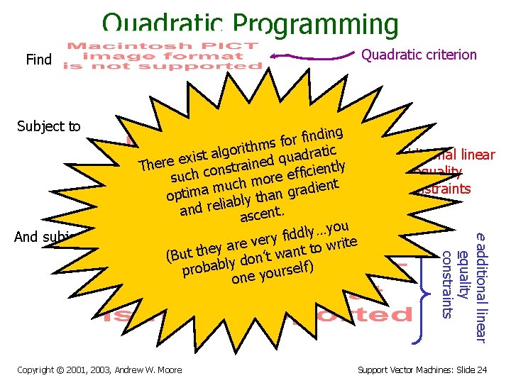
Quadratic Programming Quadratic criterion Find Subject to Copyright © 2001, 2003, Andrew W. Moore n additional linear inequality constraints e additional linear equality constraints And subject to ding n i f r o f thms i r o g l a ratic d t a s i u x q e ned i a There r t s ently n i o c i c f f h e c su more h c u ent i m d a a r m g i t op than y l b a i l and re ascent. you … y l d d i ery f v ite e r r w a o y t e t (But th ly don’t wan elf) s r probab u o y one Support Vector Machines: Slide 24

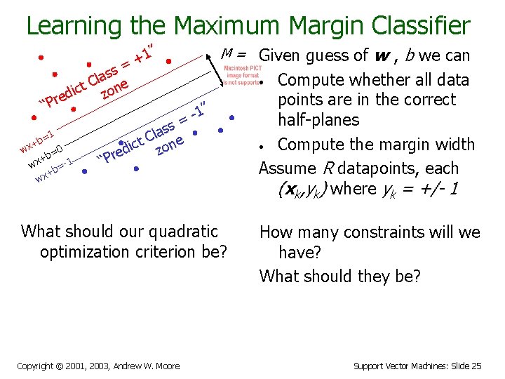
Learning the Maximum Margin Classifier ” M = Given guess of 1 + = “P +b =1 wx ss a l t C one c i z red 0 b= + wx b=-1 + wx Compute whether all data points are in the correct half-planes • Compute the margin width Assume R datapoints, each (xk, yk) where yk = +/- 1 • 1” = ss a l t C one c i z ed r P “ What should our quadratic optimization criterion be? Copyright © 2001, 2003, Andrew W. Moore w , b we can How many constraints will we have? What should they be? Support Vector Machines: Slide 25

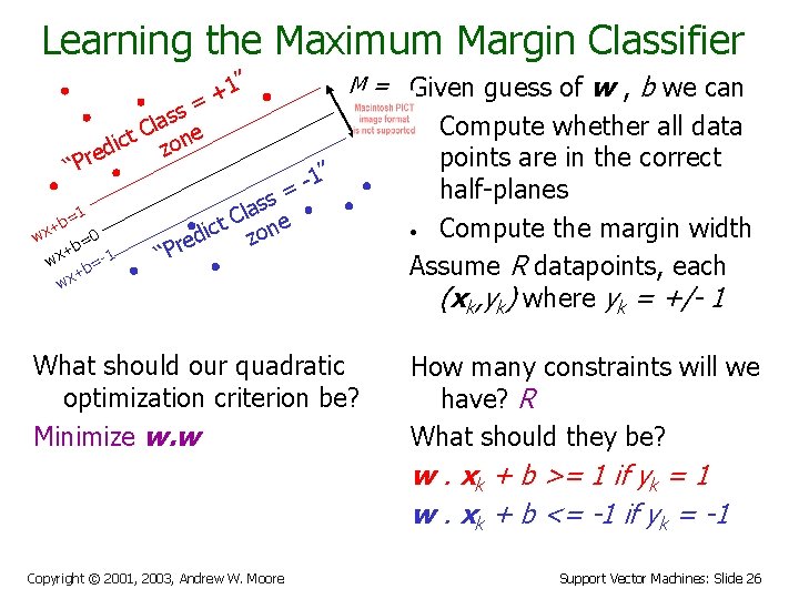
Learning the Maximum Margin Classifier ” M = Given guess of 1 + = “P +b =1 wx ss a l t C one c i z red 0 b= + wx b=-1 + wx w , b we can Compute whether all data points are in the correct half-planes • Compute the margin width Assume R datapoints, each (xk, yk) where yk = +/- 1 • 1” = ss a l t C one c i z ed r P “ What should our quadratic optimization criterion be? Minimize w. w How many constraints will we have? R What should they be? w. xk + b >= 1 if yk = 1 w. xk + b <= -1 if yk = -1 Copyright © 2001, 2003, Andrew W. Moore Support Vector Machines: Slide 26

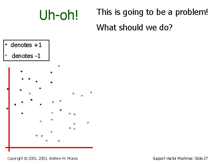
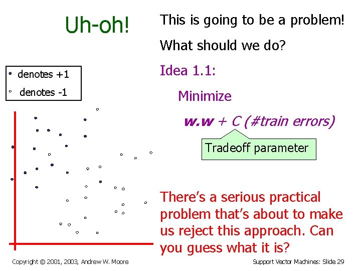
Uh-oh! This is going to be a problem! What should we do? denotes +1 denotes -1 Copyright © 2001, 2003, Andrew W. Moore Support Vector Machines: Slide 27

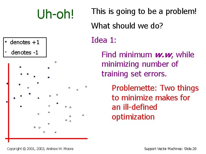
Uh-oh! denotes +1 denotes -1 This is going to be a problem! What should we do? Idea 1: Find minimum w. w, while minimizing number of training set errors. Problemette: Two things to minimize makes for an ill-defined optimization Copyright © 2001, 2003, Andrew W. Moore Support Vector Machines: Slide 28

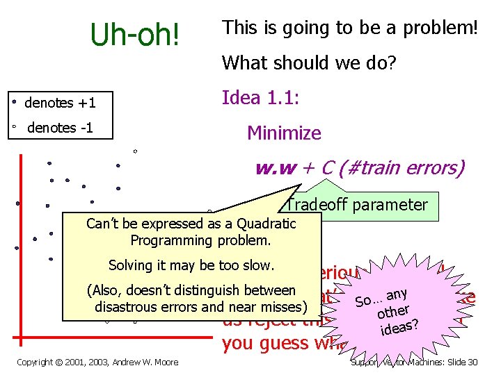
Uh-oh! denotes +1 denotes -1 This is going to be a problem! What should we do? Idea 1. 1: Minimize w. w + C (#train errors) Tradeoff parameter There’s a serious practical problem that’s about to make us reject this approach. Can you guess what it is? Copyright © 2001, 2003, Andrew W. Moore Support Vector Machines: Slide 29

Uh-oh! This is going to be a problem! What should we do? Idea 1. 1: denotes +1 denotes -1 Minimize w. w + C (#train errors) Tradeoff parameter Can’t be expressed as a Quadratic Programming problem. Solving it may be too slow. There’s a serious practical (Also, doesn’t distinguish between problem that’s about … anyto make o S disastrous errors and near misses) ther o us reject this approach. Can ideas? you guess what it is? Copyright © 2001, 2003, Andrew W. Moore Support Vector Machines: Slide 30

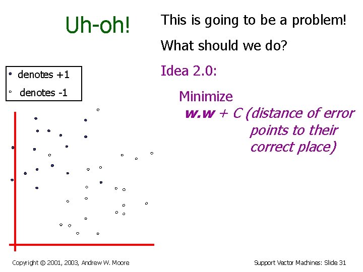
Uh-oh! denotes +1 denotes -1 This is going to be a problem! What should we do? Idea 2. 0: Minimize w. w + C (distance of error points to their correct place) Copyright © 2001, 2003, Andrew W. Moore Support Vector Machines: Slide 31

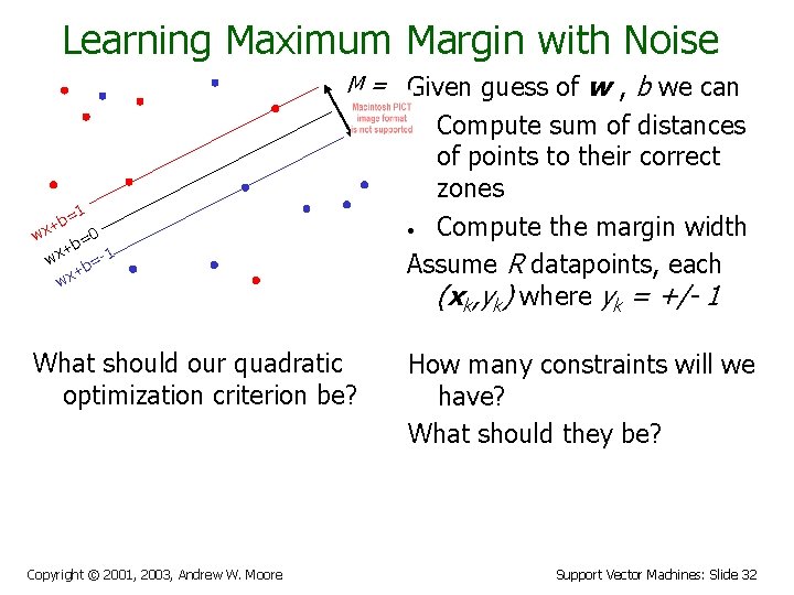
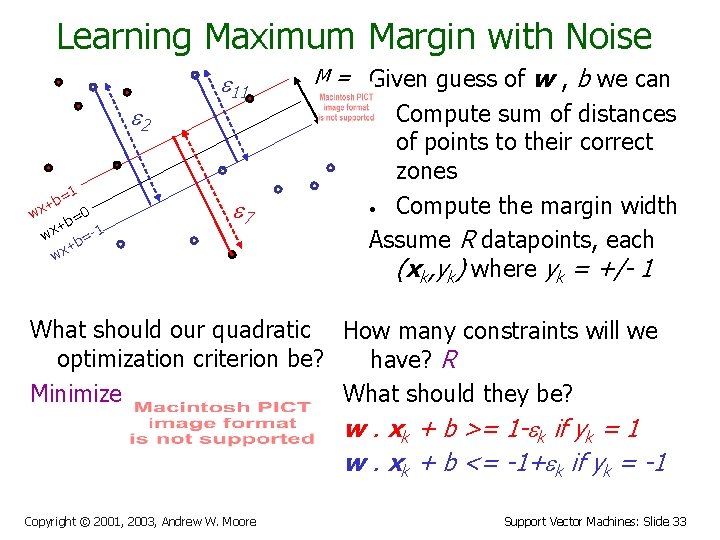
Learning Maximum Margin with Noise M = Given guess of w , b we can Compute sum of distances of points to their correct zones • Compute the margin width Assume R datapoints, each (xk, yk) where yk = +/- 1 • =1 b x+ w 0 b= + wx b=-1 + wx What should our quadratic optimization criterion be? Copyright © 2001, 2003, Andrew W. Moore How many constraints will we have? What should they be? Support Vector Machines: Slide 32

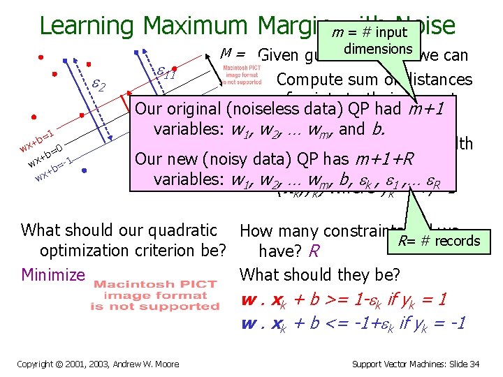
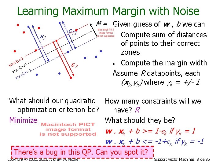
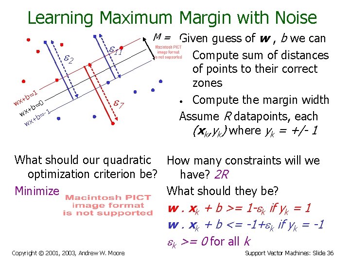
Learning Maximum Margin with Noise e 2 =1 b x+ w 0 b= + wx b=-1 + wx e 11 M = Given guess of w , b we can Compute sum of distances of points to their correct zones • Compute the margin width Assume R datapoints, each (xk, yk) where yk = +/- 1 • e 7 What should our quadratic How many constraints will we optimization criterion be? have? R Minimize What should they be? w. xk + b >= 1 -ek if yk = 1 w. xk + b <= -1+ek if yk = -1 Copyright © 2001, 2003, Andrew W. Moore Support Vector Machines: Slide 33

Learning Maximum Marginmwith Noise = # input e 2 =1 b x+ w 0 b= + wx b=-1 + wx e 11 M = Given guessdimensions of w , b we can Compute sum of distances of points to their correct Our original (noiseless data) QP had m+1 zones variables: w 1, w 2, … wm, and b. • Compute the margin width e 7 Our new (noisy data) QP has m+1+R Assume R datapoints, each variables: w 1, w 2, … wm, b, ek , e 1 , … e. R (xk, yk) where yk = +/- 1 • What should our quadratic How many constraints will we R= # records optimization criterion be? have? R Minimize What should they be? w. xk + b >= 1 -ek if yk = 1 w. xk + b <= -1+ek if yk = -1 Copyright © 2001, 2003, Andrew W. Moore Support Vector Machines: Slide 34

Learning Maximum Margin with Noise e 2 =1 b x+ w 0 b= + wx b=-1 + wx e 11 e 7 M = Given guess of w , b we can Compute sum of distances of points to their correct zones • Compute the margin width Assume R datapoints, each (xk, yk) where yk = +/- 1 • What should our quadratic How many constraints will we optimization criterion be? have? R Minimize What should they be? w. xk + b >= 1 -ek if yk = 1 w. xk + b <= -1+ek if yk = -1 There’s a bug in this QP. Can you spot it? Copyright © 2001, 2003, Andrew W. Moore Support Vector Machines: Slide 35

Learning Maximum Margin with Noise e 2 =1 b x+ w 0 b= + wx b=-1 + wx e 11 e 7 M = Given guess of w , b we can Compute sum of distances of points to their correct zones • Compute the margin width Assume R datapoints, each (xk, yk) where yk = +/- 1 • What should our quadratic How many constraints will we optimization criterion be? have? 2 R Minimize What should they be? Copyright © 2001, 2003, Andrew W. Moore w. xk + b >= 1 -ek if yk = 1 w. xk + b <= -1+ek if yk = -1 ek >= 0 for all k Support Vector Machines: Slide 36

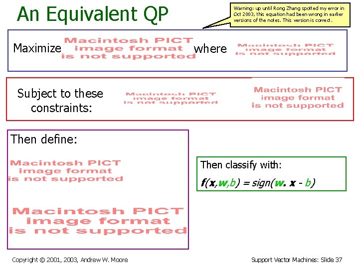
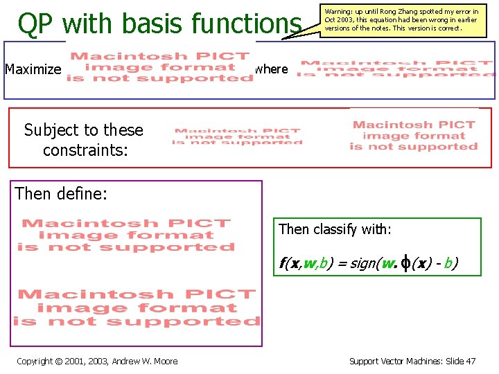
An Equivalent QP Maximize Warning: up until Rong Zhang spotted my error in Oct 2003, this equation had been wrong in earlier versions of the notes. This version is correct. where Subject to these constraints: Then define: Then classify with: f(x, w, b) = sign(w. x - b) Copyright © 2001, 2003, Andrew W. Moore Support Vector Machines: Slide 37

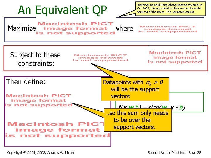
An Equivalent QP Maximize Warning: up until Rong Zhang spotted my error in Oct 2003, this equation had been wrong in earlier versions of the notes. This version is correct. where Subject to these constraints: Then define: Datapoints with ak > 0 will be the support vectors Then classify with: f(x, w, b) = sign(w. x - b) . . so this sum only needs to be over the support vectors. Copyright © 2001, 2003, Andrew W. Moore Support Vector Machines: Slide 38

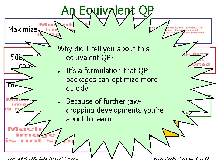
An Equivalent QP Maximize where Why did I tell you about this Subject to these equivalent QP? constraints: • It’s a formulation that QP packages can optimize more Then define: Datapoints with ak > 0 quickly • will be the support vectors Then classify with: further jaw- Because of dropping developments f(x, w, b)you’re = sign(w. x - b) about to learn. . . so this sum only needs to be over the support vectors. Copyright © 2001, 2003, Andrew W. Moore Support Vector Machines: Slide 39

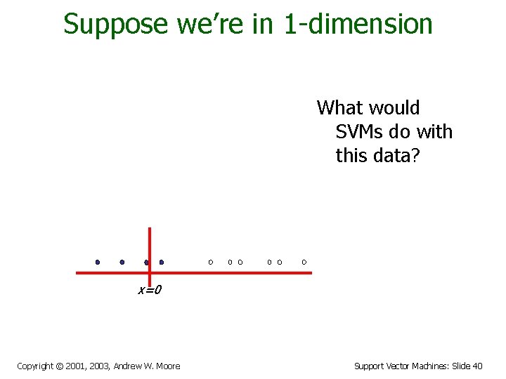
Suppose we’re in 1 -dimension What would SVMs do with this data? x=0 Copyright © 2001, 2003, Andrew W. Moore Support Vector Machines: Slide 40

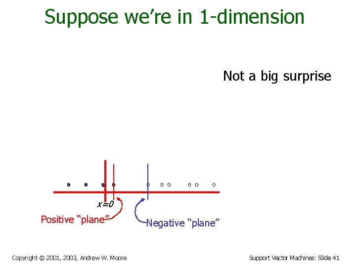
Suppose we’re in 1 -dimension Not a big surprise x=0 Positive “plane” Copyright © 2001, 2003, Andrew W. Moore Negative “plane” Support Vector Machines: Slide 41

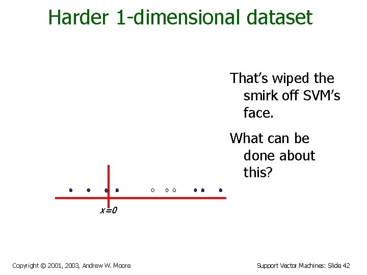
Harder 1 -dimensional dataset That’s wiped the smirk off SVM’s face. What can be done about this? x=0 Copyright © 2001, 2003, Andrew W. Moore Support Vector Machines: Slide 42

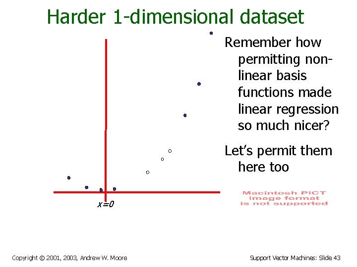
Harder 1 -dimensional dataset Remember how permitting nonlinear basis functions made linear regression so much nicer? Let’s permit them here too x=0 Copyright © 2001, 2003, Andrew W. Moore Support Vector Machines: Slide 43

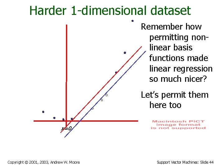
Harder 1 -dimensional dataset Remember how permitting nonlinear basis functions made linear regression so much nicer? Let’s permit them here too x=0 Copyright © 2001, 2003, Andrew W. Moore Support Vector Machines: Slide 44

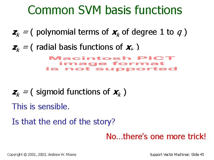
Common SVM basis functions zk = ( polynomial terms of xk of degree 1 to q ) zk = ( radial basis functions of xk ) zk = ( sigmoid functions of xk ) This is sensible. Is that the end of the story? No…there’s one more trick! Copyright © 2001, 2003, Andrew W. Moore Support Vector Machines: Slide 45

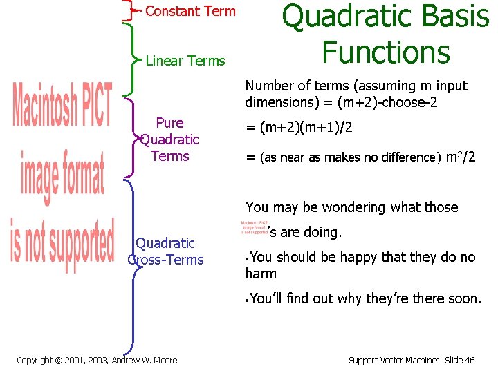
Quadratic Basis Functions Constant Term Linear Terms Number of terms (assuming m input dimensions) = (m+2)-choose-2 Pure Quadratic Terms = (m+2)(m+1)/2 = (as near as makes no difference) m 2/2 You may be wondering what those Quadratic Cross-Terms ’s are doing. You should be happy that they do no harm • You’ll find out why they’re there soon. • Copyright © 2001, 2003, Andrew W. Moore Support Vector Machines: Slide 46

QP with basis functions Maximize Warning: up until Rong Zhang spotted my error in Oct 2003, this equation had been wrong in earlier versions of the notes. This version is correct. where Subject to these constraints: Then define: Then classify with: f(x, w, b) = sign(w. f(x) - b) Copyright © 2001, 2003, Andrew W. Moore Support Vector Machines: Slide 47

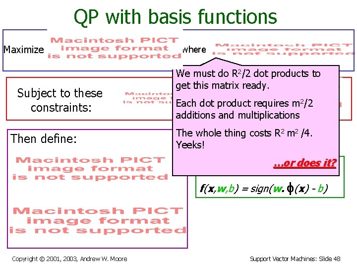
QP with basis functions Maximize Subject to these constraints: Then define: where We must do R 2/2 dot products to get this matrix ready. Each dot product requires m 2/2 additions and multiplications The whole thing costs R 2 m 2 /4. Yeeks! …or does it? Then classify with: f(x, w, b) = sign(w. f(x) - b) Copyright © 2001, 2003, Andrew W. Moore Support Vector Machines: Slide 48

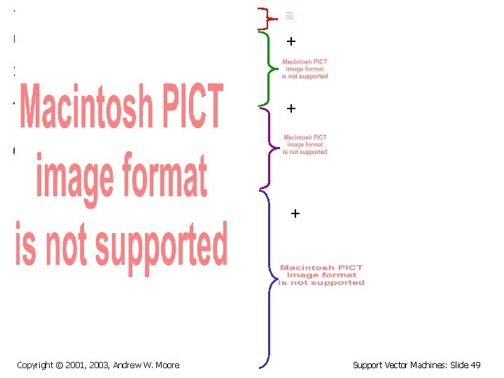
Quadratic Dot Products + + + Copyright © 2001, 2003, Andrew W. Moore Support Vector Machines: Slide 49

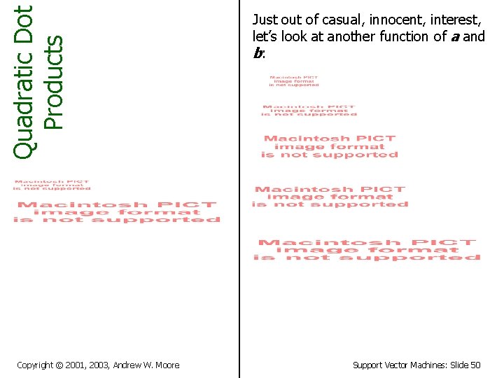
Quadratic Dot Products Copyright © 2001, 2003, Andrew W. Moore Just out of casual, innocent, interest, let’s look at another function of a and b: Support Vector Machines: Slide 50

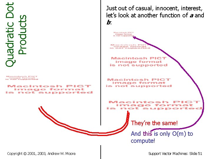
Quadratic Dot Products Just out of casual, innocent, interest, let’s look at another function of a and b: They’re the same! And this is only O(m) to compute! Copyright © 2001, 2003, Andrew W. Moore Support Vector Machines: Slide 51

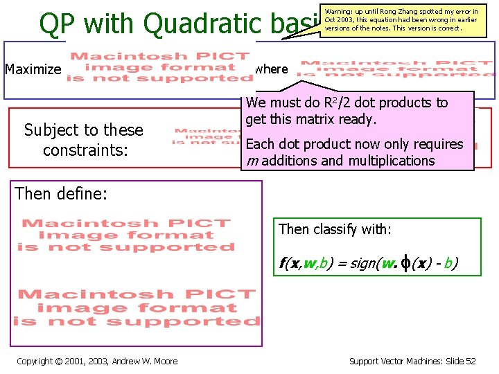
QP with Quadratic basis functions Warning: up until Rong Zhang spotted my error in Oct 2003, this equation had been wrong in earlier versions of the notes. This version is correct. Maximize Subject to these constraints: where We must do R 2/2 dot products to get this matrix ready. Each dot product now only requires m additions and multiplications Then define: Then classify with: f(x, w, b) = sign(w. f(x) - b) Copyright © 2001, 2003, Andrew W. Moore Support Vector Machines: Slide 52

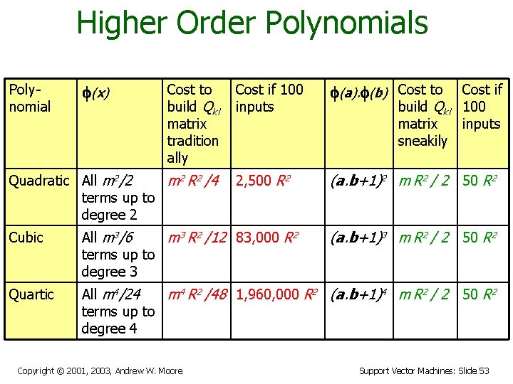
Higher Order Polynomials Polynomial f(x) Cost to build Qkl matrix tradition ally Quadratic All m 2/2 m 2 R 2 /4 terms up to degree 2 Cost if 100 inputs f(a). f(b) Cost to 2, 500 R 2 (a. b+1)2 m R 2 / 2 50 R 2 build Qkl matrix sneakily Cubic All m 3/6 m 3 R 2 /12 83, 000 R 2 terms up to degree 3 Quartic All m 4/24 m 4 R 2 /48 1, 960, 000 R 2 (a. b+1)4 m R 2 / 2 terms up to degree 4 Copyright © 2001, 2003, Andrew W. Moore Cost if 100 inputs (a. b+1)3 m R 2 / 2 50 R 2 Support Vector Machines: Slide 53

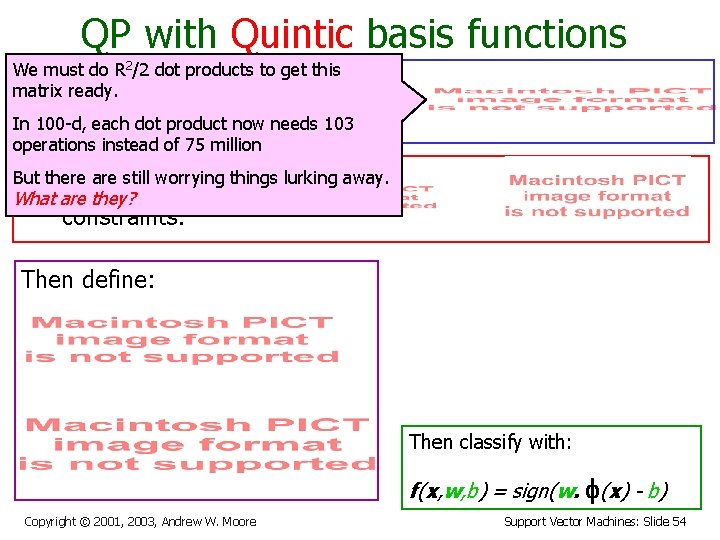
QP with Quintic basis functions We must do R 2/2 dot products to get this matrix ready. Maximize where In 100 -d, each dot product now needs 103 operations instead of 75 million But there are still worrying things lurking away. Subject to What are they? these constraints: Then define: Then classify with: f(x, w, b) = sign(w. f(x) - b) Copyright © 2001, 2003, Andrew W. Moore Support Vector Machines: Slide 54

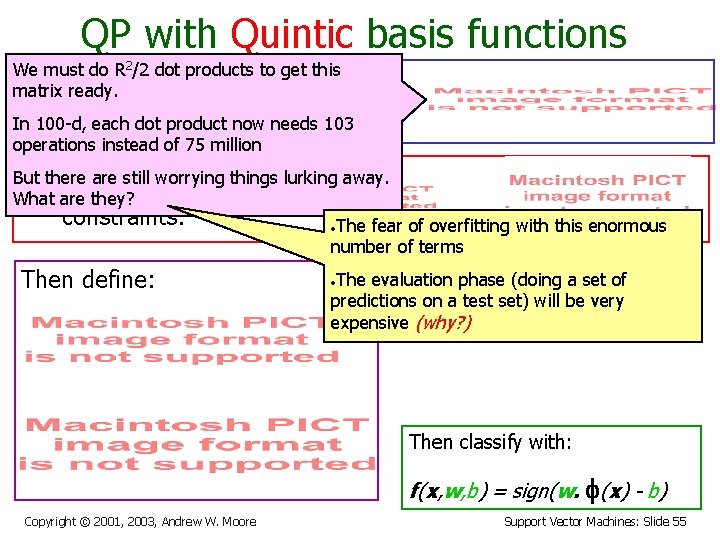
QP with Quintic basis functions We must do R 2/2 dot products to get this matrix ready. Maximize where In 100 -d, each dot product now needs 103 operations instead of 75 million But there are still worrying things lurking away. Subject to these What are they? constraints: • The fear of overfitting with this enormous number of terms Then define: • The evaluation phase (doing a set of predictions on a test set) will be very expensive (why? ) Then classify with: f(x, w, b) = sign(w. f(x) - b) Copyright © 2001, 2003, Andrew W. Moore Support Vector Machines: Slide 55

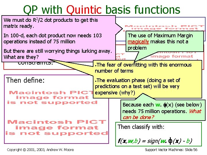
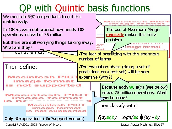
QP with Quintic basis functions We must do R 2/2 dot products to get this matrix ready. Maximize In 100 -d, each dot product now needs 103 operations instead of 75 million where The use of Maximum Margin magically makes this not a problem But there are still worrying things lurking away. Subject to these What are they? constraints: • The fear of overfitting with this enormous number of terms Then define: • The evaluation phase (doing a set of predictions on a test set) will be very expensive (why? ) Because each w. f(x) (see below) needs 75 million operations. What can be done? Then classify with: f(x, w, b) = sign(w. f(x) - b) Copyright © 2001, 2003, Andrew W. Moore Support Vector Machines: Slide 56

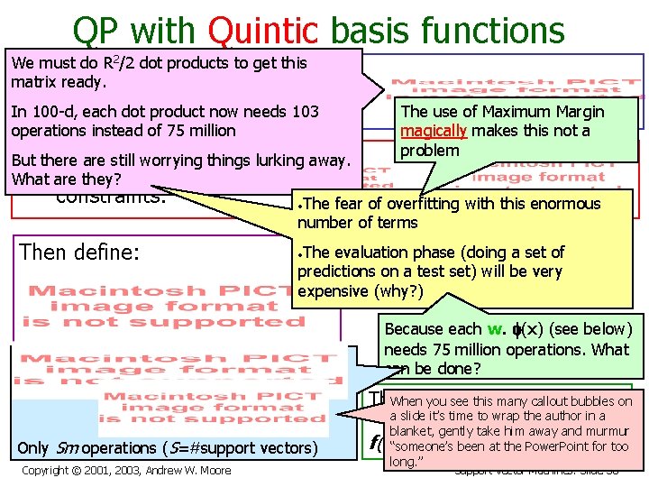
QP with Quintic basis functions We must do R 2/2 dot products to get this matrix ready. Maximize In 100 -d, each dot product now needs 103 operations instead of 75 million where The use of Maximum Margin magically makes this not a problem But there are still worrying things lurking away. Subject to these What are they? constraints: • The fear of overfitting with this enormous number of terms Then define: • The evaluation phase (doing a set of predictions on a test set) will be very expensive (why? ) Because each w. f(x) (see below) needs 75 million operations. What can be done? Then classify with: Only Sm operations (S=#support vectors) Copyright © 2001, 2003, Andrew W. Moore f(x, w, b) = sign(w. f(x) - b) Support Vector Machines: Slide 57

QP with Quintic basis functions We must do R 2/2 dot products to get this matrix ready. Maximize In 100 -d, each dot product now needs 103 operations instead of 75 million where The use of Maximum Margin magically makes this not a problem But there are still worrying things lurking away. Subject to these What are they? constraints: • The fear of overfitting with this enormous number of terms Then define: • The evaluation phase (doing a set of predictions on a test set) will be very expensive (why? ) Because each w. f(x) (see below) needs 75 million operations. What can be done? Then classify with: When you see this many callout bubbles on Only Sm operations (S=#support vectors) Copyright © 2001, 2003, Andrew W. Moore a slide it’s time to wrap the author in a blanket, gently take him away and murmur f(x, w, b) = been sign(w. (x) - b)for too “someone’s at the Power. Point long. ” f Support Vector Machines: Slide 58

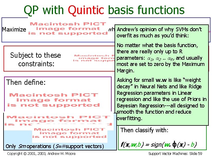
QP with Quintic basis functions Maximize Subject to these constraints: Then define: where Andrew’s opinion of why SVMs don’t overfit as much as you’d think: No matter what the basis function, there are really only up to R parameters: a 1, a 2. . a. R, and usually most are set to zero by the Maximum Margin. Asking for small w. w is like “weight decay” in Neural Nets and like Ridge Regression parameters in Linear regression and like the use of Priors in Bayesian Regression---all designed to smooth the function and reduce overfitting. Then classify with: Only Sm operations (S=#support vectors) Copyright © 2001, 2003, Andrew W. Moore f(x, w, b) = sign(w. f(x) - b) Support Vector Machines: Slide 59

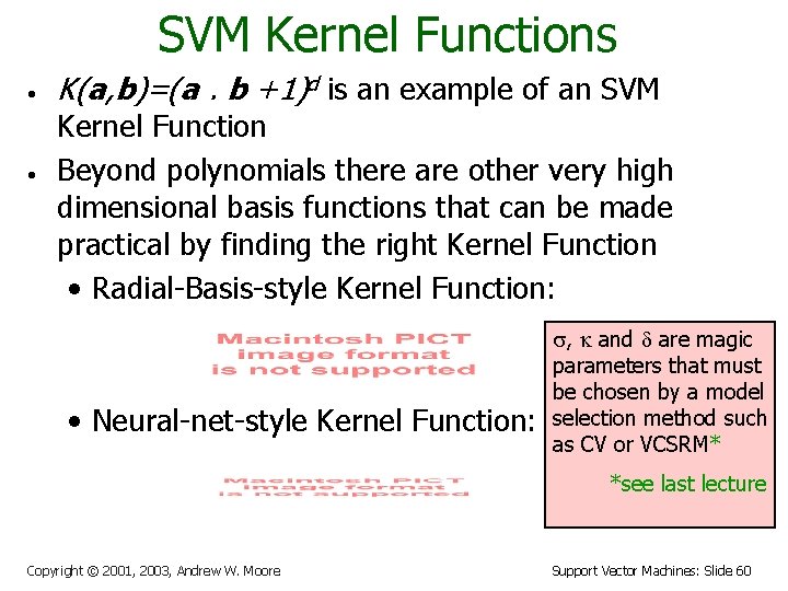
SVM Kernel Functions • • K(a, b)=(a. b +1)d is an example of an SVM Kernel Function Beyond polynomials there are other very high dimensional basis functions that can be made practical by finding the right Kernel Function • Radial-Basis-style Kernel Function: • Neural-net-style Kernel Function: s, k and d are magic parameters that must be chosen by a model selection method such as CV or VCSRM* *see last lecture Copyright © 2001, 2003, Andrew W. Moore Support Vector Machines: Slide 60

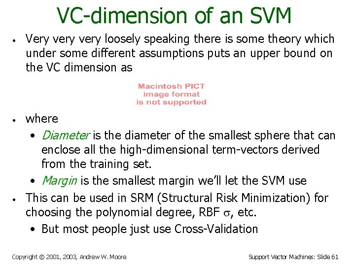
VC-dimension of an SVM • • • Very very loosely speaking there is some theory which under some different assumptions puts an upper bound on the VC dimension as where • Diameter is the diameter of the smallest sphere that can enclose all the high-dimensional term-vectors derived from the training set. • Margin is the smallest margin we’ll let the SVM use This can be used in SRM (Structural Risk Minimization) for choosing the polynomial degree, RBF s, etc. • But most people just use Cross-Validation Copyright © 2001, 2003, Andrew W. Moore Support Vector Machines: Slide 61

SVM Performance • • • Anecdotally they work very well indeed. Example: They are currently the best-known classifier on a well-studied hand-written-character recognition benchmark Another Example: Andrew knows several reliable people doing practical real-world work who claim that SVMs have saved them when their other favorite classifiers did poorly. There is a lot of excitement and religious fervor about SVMs as of 2001. Despite this, some practitioners (including your lecturer) are a little skeptical. Copyright © 2001, 2003, Andrew W. Moore Support Vector Machines: Slide 62

Doing multi-classification • • • SVMs can only handle two-class outputs (i. e. a categorical output variable with arity 2). What can be done? Answer: with output arity N, learn N SVM’s • • • SVM 1 learns “Output==1” vs “Output != 1” SVM 2 learns “Output==2” vs “Output != 2” : SVM N learns “Output==N” vs “Output != N” Then to predict the output for a new input, just predict with each SVM and find out which one puts the prediction the furthest into the positive region. Copyright © 2001, 2003, Andrew W. Moore Support Vector Machines: Slide 63

References • An excellent tutorial on VC-dimension and Support Vector Machines: C. J. C. Burges. A tutorial on support vector machines for pattern recognition. Data Mining and Knowledge Discovery, 2(2): 955 -974, 1998. http: //citeseer. nj. nec. com/burges 98 tutorial. html • The VC/SRM/SVM Bible: Statistical Learning Theory by Vladimir Vapnik, Wiley. Interscience; 1998 Copyright © 2001, 2003, Andrew W. Moore Support Vector Machines: Slide 64

What You Should Know • • Linear SVMs The definition of a maximum margin classifier What QP can do for you (but, for this class, you don’t need to know how it does it) How Maximum Margin can be turned into a QP problem How we deal with noisy (non-separable) data How we permit non-linear boundaries How SVM Kernel functions permit us to pretend we’re working with ultra-high-dimensional basisfunction terms Copyright © 2001, 2003, Andrew W. Moore Support Vector Machines: Slide 65