Support for Dymola in the Modeling and Simulation

Support for Dymola in the Modeling and Simulation of Physical Systems with Distributed Parameters Student: Dshabarow Farid Professor: Prof. François Cellier Verantwortlich: Prof. Walter Gander

Outline n n n n n Objectives of the Master Thesis Building Blocks Dymola and Modelica Partial Differential Equations Method of Lines Finite Volume Method General Block Conclusion Literature

Objectives of the Master Thesis n Create blocks in Dymola that can be used to „construct“ partial differential equations (PDEs) and implement numerical methods to solve them n Numerical Methods: n n n Method of Lines Finite Volume Method Adaptive Method of Lines

Building Blocks: PDE n PDE Blocks Which blocks do we need for PDEs? For example: n n n Derivator Block Integrator Blocks for Addition, Subtraction, Product, . . .

Building Blocks: PDE n PDE Construction After we have the blocks, we can use them to construct PDEs

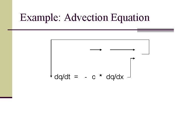
Example: Advection Equation dq/dt = - c * dq/dx

Example: Advection Equation

Dymola & Modelica n Dymola (Dynamic Modeling Laboratory) is an integrated environment for the modeling and simulation of physical systems in Modelica language n Modelica is a general, high-level language for object- oriented modeling with differential-algebraic equations n Dymola provides standard blocks like sum, product, division, . . .

PDE Library n Provides necessary blocks for the PDEs „construction“ and numerical methods for their solution n Implements new blocks and uses standard blocks provided by Modelica n Two numerical methods are provided for solving PDEs: n n Method of Lines Finite Volume Methods

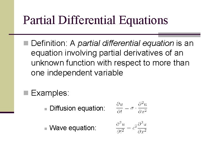
Partial Differential Equations n Definition: A partial differential equation is an equation involving partial derivatives of an unknown function with respect to more than one independent variable n Examples: n Diffusion equation: n Wave equation:

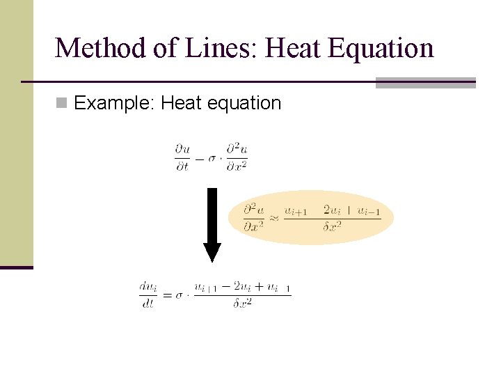
Method of Lines (1 D) n The Method of Lines (MOL) solves numerically a PDE by discretizing the space variable but leaving the time variable continuous n We are thus converting a PDE into a set of Ordinary Differential Equations (ODEs)! n Advantage: efficient ODE solvers are known

Method of Lines: Heat Equation n Example: Heat equation

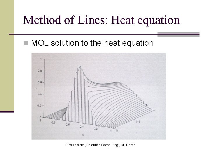
Method of Lines: Heat equation n MOL solution to the heat equation Picture from „Scientific Computing“, M. Heath

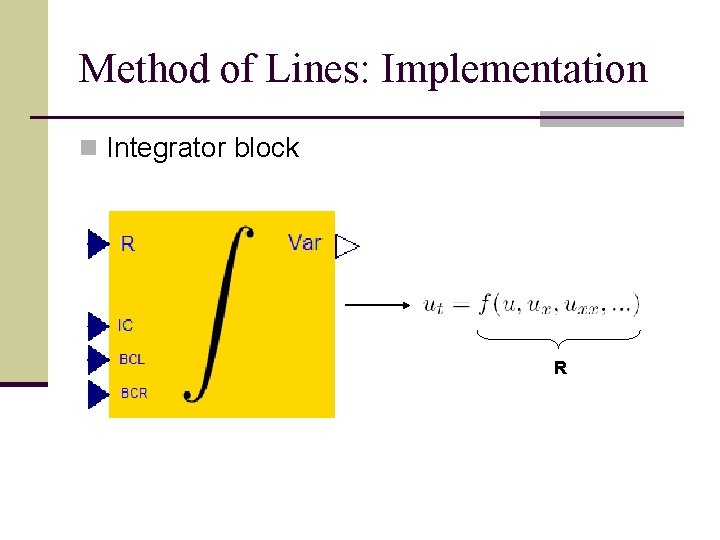
Method of Lines: Implementation n Integrator block R

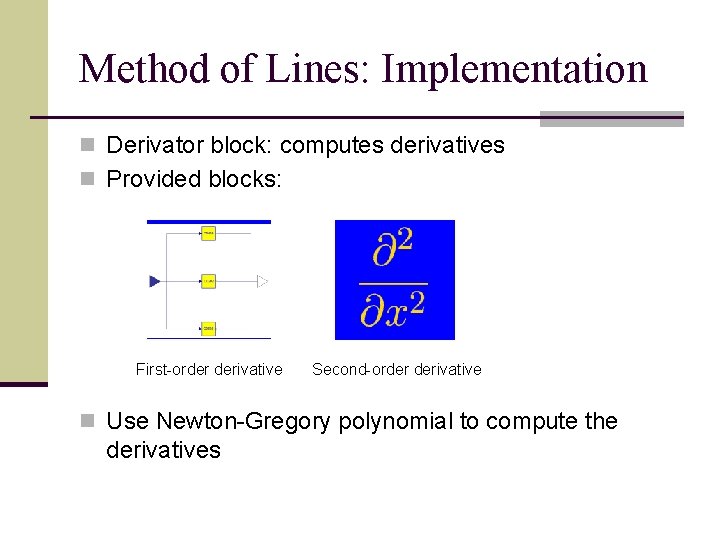
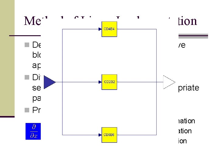
Method of Lines: Implementation n Derivator block: computes derivatives n Provided blocks: First-order derivative Second-order derivative n Use Newton-Gregory polynomial to compute the derivatives

Method of Lines: Implementation n Derivator block: includes three derivative blocks, each with different order of approximation accuracy n Different approximation orders can be selected by the user through the appropriate parameter n Provided approximation orders: n n n Second-order central difference approximation Fourth-order central difference approximation Sixth-order central difference approximation

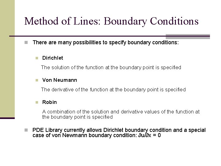
Method of Lines: Boundary Conditions n There are many possibilities to specify boundary conditions: n Dirichlet The solution of the function at the boundary point is specified n Von Neumann The derivative of the function at the boundary point is specified n Robin A combination of the solution and derivative values of the function at the boundary point is specified n PDE Library currently allows Dirichlet boundary condition and a special case of von Newmann boundary condition: ∂u/∂x = 0

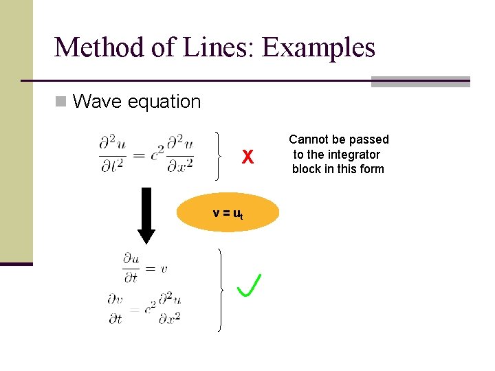
Method of Lines: Examples n Wave equation X v = ut Cannot be passed to the integrator block in this form

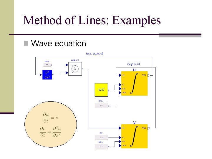
Method of Lines: Examples n Wave equation

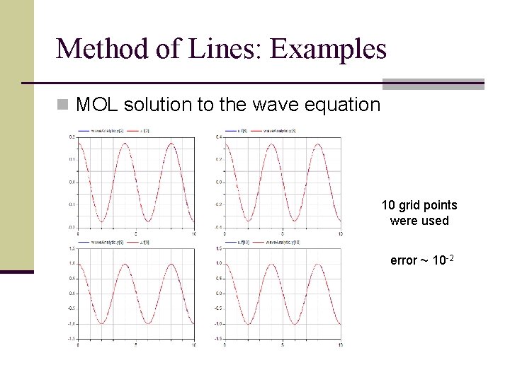
Method of Lines: Examples n MOL solution to the wave equation 10 grid points were used error ~ 10 -2

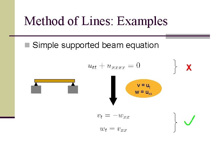
Method of Lines: Examples n Simple supported beam equation X v = ut w = uxx

Method of Lines: Examples n Simple supported beam equation

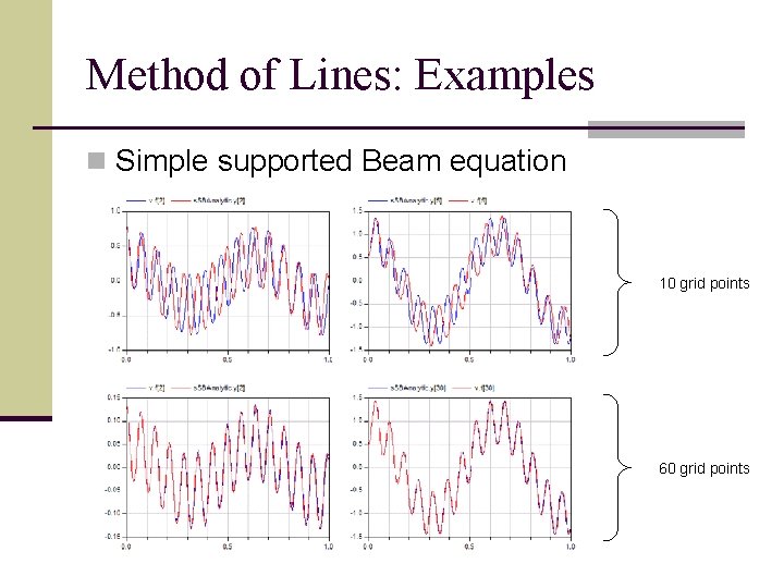
Method of Lines: Examples n Simple supported Beam equation 10 grid points 60 grid points

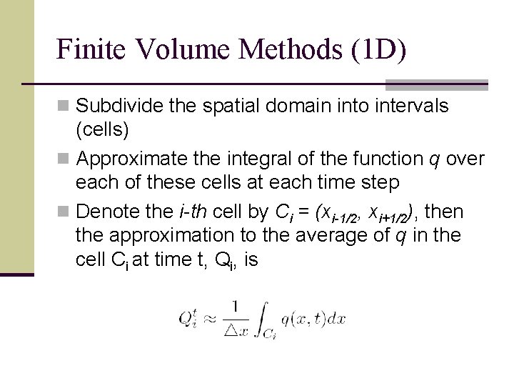
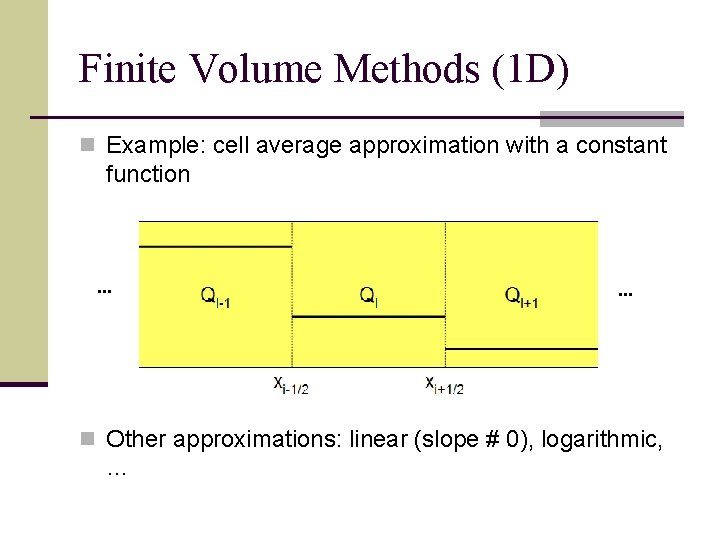
Finite Volume Methods (1 D) n Subdivide the spatial domain into intervals (cells) n Approximate the integral of the function q over each of these cells at each time step n Denote the i-th cell by Ci = (xi-1/2, xi+1/2), then the approximation to the average of q in the cell Ci at time t, Qi, is

Finite Volume Methods (1 D) n Example: cell average approximation with a constant function . . . n Other approximations: linear (slope # 0), logarithmic, …

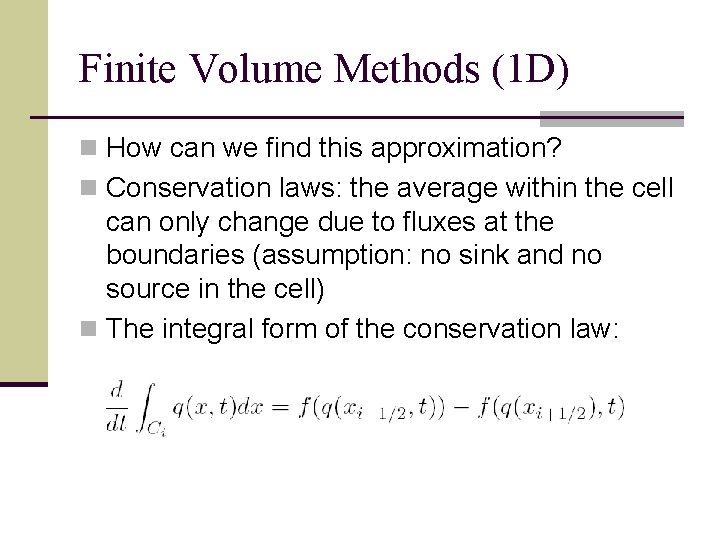
Finite Volume Methods (1 D) n How can we find this approximation? n Conservation laws: the average within the cell can only change due to fluxes at the boundaries (assumption: no sink and no source in the cell) n The integral form of the conservation law:

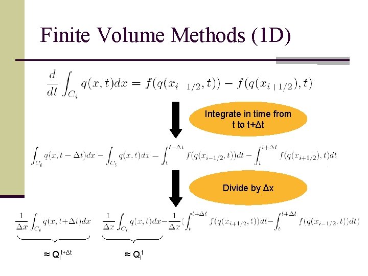
Finite Volume Methods (1 D) Integrate in time from t to t+Δt Divide by Δx ≈ Qit+Δt ≈ Qit

Finite Volume Methods (1 D) n Average update rule where approximates the average flux along xi-1/2

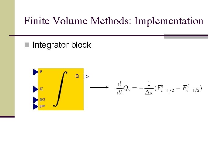
Finite Volume Methods (1 D) n The average update rule can also be written in this form n We have thus an ODE for each cell!

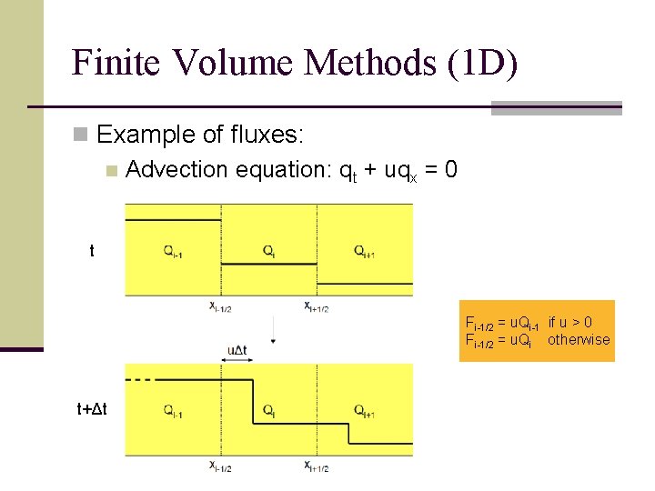
Finite Volume Methods (1 D) n Example of fluxes: n Advection equation: qt + uqx = 0 t Fi-1/2 = u. Qi-1 if u > 0 Fi-1/2 = u. Qi otherwise t+Δt

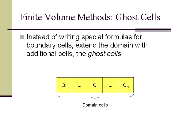
Finite Volume Methods: Ghost Cells n Instead of writing special formulas for boundary cells, extend the domain with additional cells, the ghost cells

Finite Volume Methods: Implementation n Integrator block

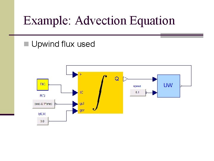
Finite Volume Methods: Implementation n Flux block: Upwind Fi-1/2 = u. Qi-1 if u > 0 Fi-1/2 = u. Qi if u < 0 u

Example: Advection Equation n Upwind flux used

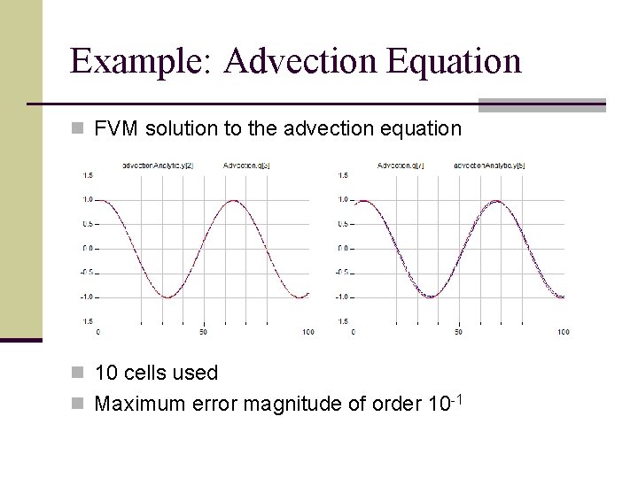
Example: Advection Equation n FVM solution to the advection equation n 10 cells used n Maximum error magnitude of order 10 -1

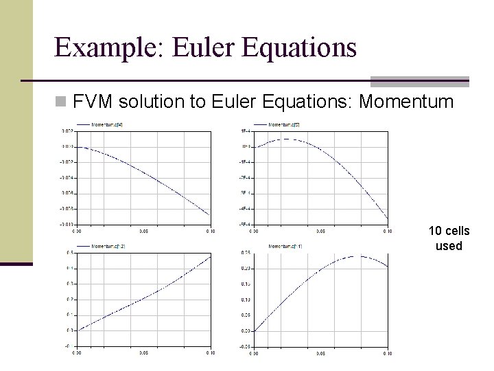
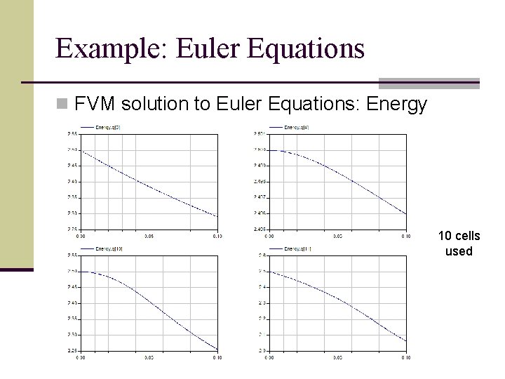
Example: Euler Equations n Fluids (liquids and gases) are governed by conservation laws: Conservation of mass n Conservation of momentum n Conservation of energy n n The resulting system of 3 equations gives the Euler equations of gas dynamics

Example: Euler Equations n How do these equations look like? It depends on the chosen model n Two fundamental ways to derive the equations: Eulerian approach n Lagrangian approach n

Example: Euler Equations n Consider for ex. the velocity field n Eulerian description: n Describes the behavior of the velocity field at a particular point over time n Lagrangian description: n Describes the behavior of the velocity of the particles as they move through the flow

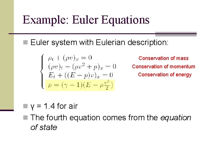
Example: Euler Equations n Euler system with Eulerian description: Conservation of mass Conservation of momentum Conservation of energy n γ = 1. 4 for air n The fourth equation comes from the equation of state

Example: Euler Equations Logarithmic Reconstruction

Example: Euler Equations n FVM solution to Euler Equations: Density 10 cells used

Example: Euler Equations n FVM solution to Euler Equations: Momentum 10 cells used

Example: Euler Equations n FVM solution to Euler Equations: Energy 10 cells used

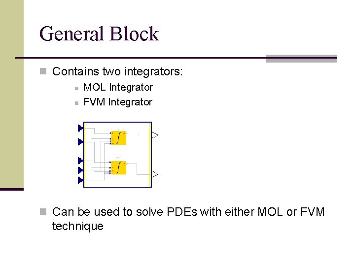
General Block n Contains two integrators: n MOL Integrator n FVM Integrator n Can be used to solve PDEs with either MOL or FVM technique

Conclusion n Method of Lines n Simple to implement n Gives accurate results n Not suited for the simulation of Euler equations (spurious oscillations) n Finite Volume Method n Poor Literature n Complicated theory n Equations must be rewritten in conservation form n First-order methods are not as accurate as Method of Lines n Better suited for the simulation of Euler equations

Literature n Stanley J. Farlow: Partial Differential Equations for Scientists and Engineers n François E. Cellier, Ernesto Kofman: Continous System Simulation n Randall J. Leveque: Finite Volume Methods for Hyperbolic Problems n John D. Anderson: Computational Fluid Dynamics

QUESTIONS?