Supply Curve Basics Unit 7 Producers and Supply

Supply Curve Basics Unit 7: Producers and Supply

I. Supply supply – the amount of a good that people are willing and able to sell at every possible price • economists differentiate between supply and quantity supplied in the same manner as with demand

II. Law of Supply law of demand – the quantity supplied of a good increases as price rises and decreases as price falls • there is a direct relationship between price and quantity: Price↓, Quantity↓ Price↑, Quantity↑ • same assumptions for law of demand to be true must also be made for law of supply to be true

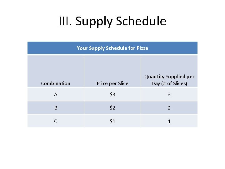
III. Supply Schedule Your Supply Schedule for Pizza Combination Price per Slice Quantity Supplied per Day (# of Slices) A $3 3 B $2 2 C $1 1

IV. Supply Curve • same characteristics as for demand curve except the slope is always positive because of the direct relationship between price and quantity

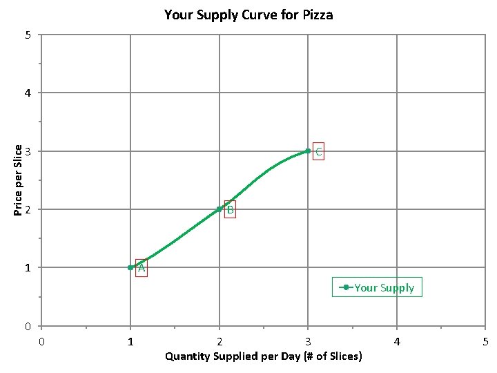
Your Supply Curve for Pizza 5 Price per Slice 4 3 C B 2 1 A Your Supply 0 0 1 2 3 Quantity Supplied per Day (# of Slices) 4 5

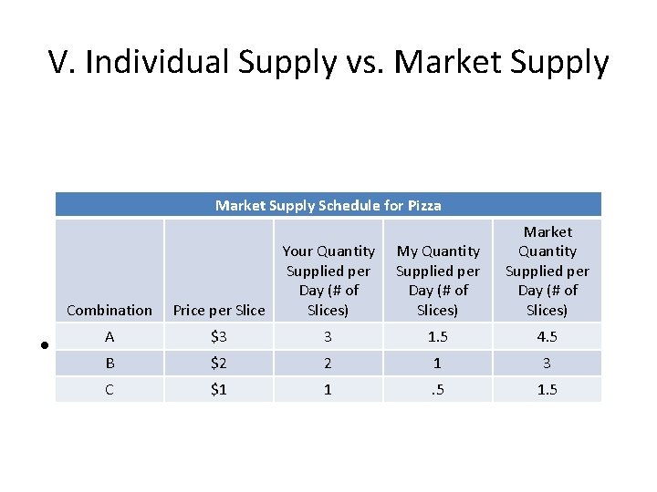
V. Individual Supply vs. Market Supply Schedule for Pizza Combination Price per Slice Your Quantity Supplied per Day (# of Slices) A $3 3 My Quantity Supplied per Day (# of Slices) Market Quantity Supplied per Day (# of Slices) 1. 5 4. 5 • note. B that each individual can have a different $2 2 1 3 demand for the same 1 good C $1. 5

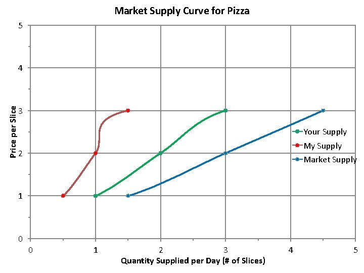
Market Supply Curve for Pizza 5 Price per Slice 4 3 Your Supply My Supply 2 Market Supply 1 0 0 1 2 3 Quantity Supplied per Day (# of Slices) 4 5

VI. Changes in Quantity Supplied vs. Changes in Supply • same principles as demand: – price changes affect quantity supplied and there will be movement along supply curve – other variables affect supply and there will be shifts of the entire supply curve

Your Supply Curve for Pizza 5 Price per Slice 4 3 C B 2 1 A Your Supply 0 0 1 2 3 Quantity Supplied per Day (# of Slices) 4 5

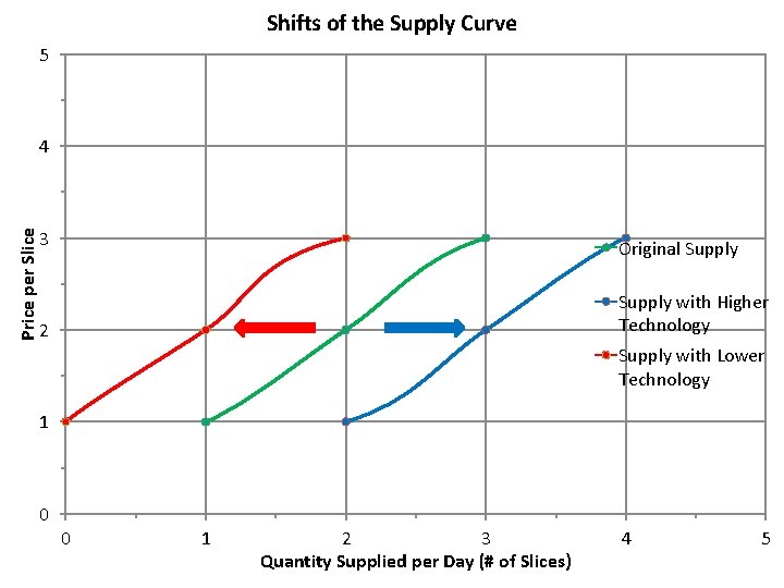
Shifts of the Supply Curve 5 Price per Slice 4 3 Original Supply 2 Supply with Higher Technology Supply with Lower Technology 1 0 0 1 2 3 Quantity Supplied per Day (# of Slices) 4 5

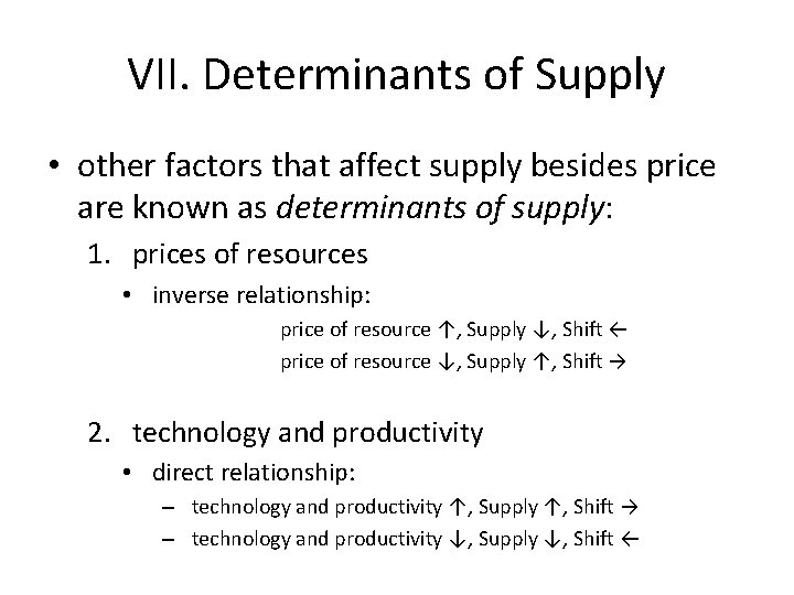
VII. Determinants of Supply • other factors that affect supply besides price are known as determinants of supply: 1. prices of resources • inverse relationship: price of resource ↑, Supply ↓, Shift ← price of resource ↓, Supply ↑, Shift → 2. technology and productivity • direct relationship: – technology and productivity ↑, Supply ↑, Shift → – technology and productivity ↓, Supply ↓, Shift ←

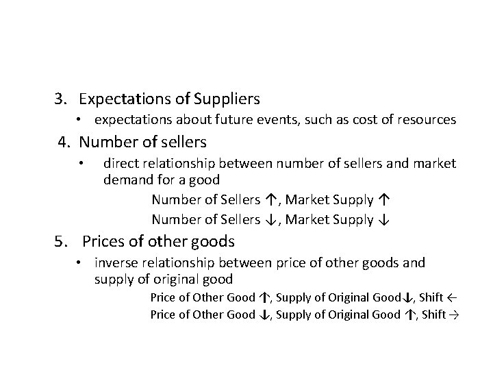
3. Expectations of Suppliers • expectations about future events, such as cost of resources 4. Number of sellers • direct relationship between number of sellers and market demand for a good Number of Sellers ↑, Market Supply ↑ Number of Sellers ↓, Market Supply ↓ 5. Prices of other goods • inverse relationship between price of other goods and supply of original good Price of Other Good ↑, Supply of Original Good↓, Shift ← Price of Other Good ↓, Supply of Original Good ↑, Shift →

VIII. Elasticity of Supply • measures sensitivity of supply to changes in any variable that affects supply: – ex: price elasticity of supply – calculated same as for demand – whatever kind of elasticity, dependent variable (Q) is always the numerator, and the independent variable (P) is always the denominator

IX. Determinants of Price Elasticity of Supply 1. short-run vs. long-run – in the short-run, firms can’t adjust their resources to alter their supply given changes in prices, so supply tends to be more inelastic – in the long-run, firms can adjust and alter their supply given changes in prices so supply tends to more elastic

The Upward Slope of the Supply Curve I: Physical Product Unit 7: Producers and Supply

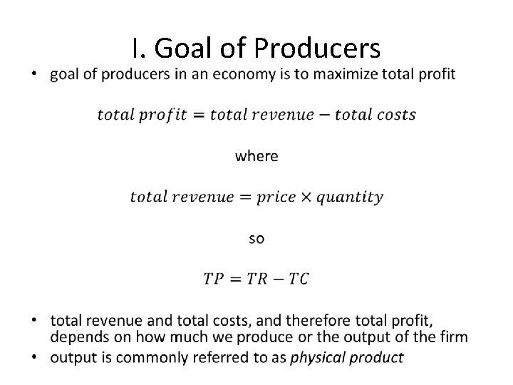
I. Goal of Producers •

II. The Production Function production function – schedule showing the physical product (output) that can be produced given different quantities of resources (inputs) • in the short-run, most resources are fixed and cannot be changed • labor usually can be changed and is therefore a variable resource

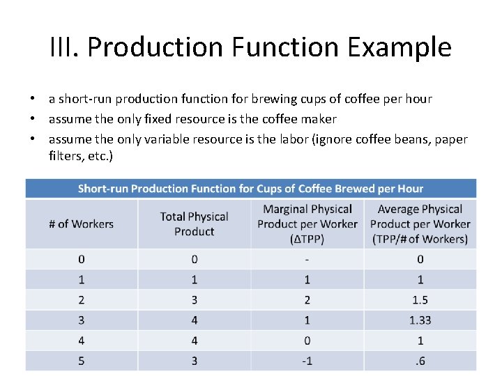
III. Production Function Example • a short-run production function for brewing cups of coffee per hour • assume the only fixed resource is the coffee maker • assume the only variable resource is the labor (ignore coffee beans, paper filters, etc. )

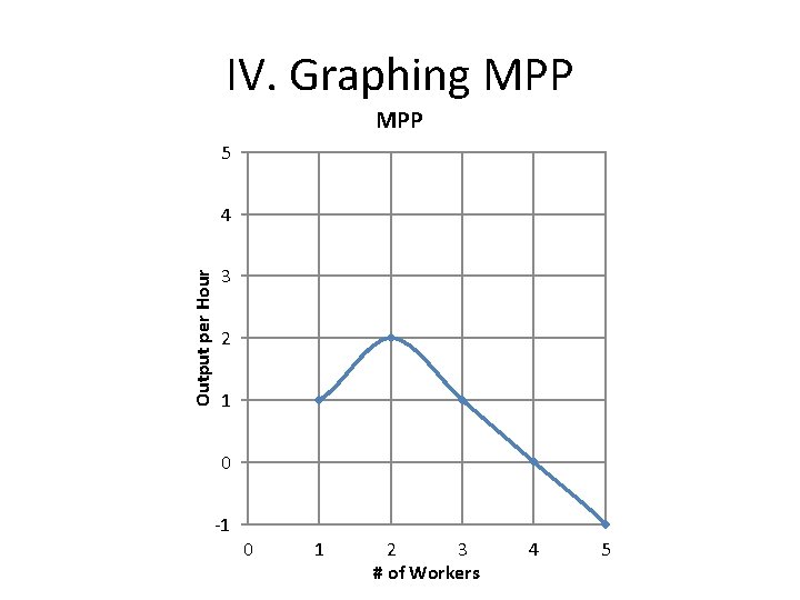
IV. Graphing MPP 5 Output per Hour 4 3 2 1 0 -1 0 1 2 3 # of Workers 4 5

V. Law of Diminishing Marginal Product or Returns • at first, an additional worker (the second) increases productivity compared to the first, but then each additional worker just gets in the way when there’s only one coffee maker and actually decreases productivity law of diminishing marginal product – when successive equal amounts of a variable resource are combined with a fixed amount of another resource, marginal product will at first increase and then decrease

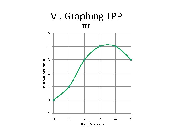
VI. Graphing TPP 5 output per Hour 4 3 2 1 0 -1 0 1 2 3 # of Workers 4 5

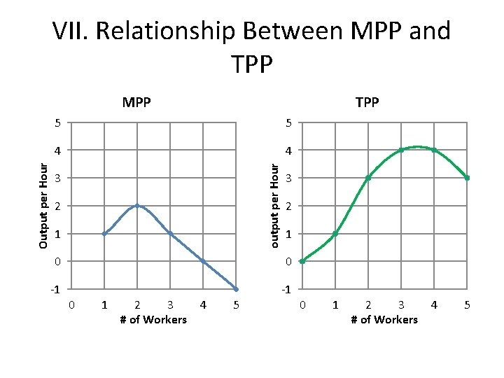
VII. Relationship Between MPP and TPP 5 5 4 4 output per Hour Output per Hour MPP 3 2 1 0 0 -1 -1 0 1 2 3 # of Workers 4 5

• as long as MPP is +, TPP will increase • if MPP is + and is increasing, TPP will increase at an increasing rate • if MPP is + and is decreasing, TPP will increase at a decreasing rate • if MPP is 0, TPP will remain constant • if MPP becomes -, TPP will decrease • all of this will happen in that order according to the law of diminishing marginal product

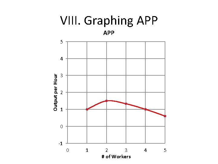
VIII. Graphing APP 5 Output per Hour 4 3 2 1 0 -1 0 1 2 3 # of Workers 4 5

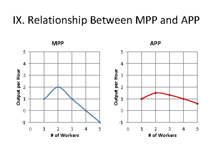
IX. Relationship Between MPP and APP 5 5 4 4 Output per Hour MPP 3 2 1 0 0 -1 -1 0 1 2 3 # of Workers 4 5

• as long as MPP is above the APP, the APP will be rising • as long as the MPP is below the APP, the APP will be falling • this makes sense, think of MPP as your last quarter’s GPA and APP as your average GPA • if this quarter’s is above your previous average, then it will pull up your average, • if this quarter’s is below your previous average, then it will pull down your average • therefore, the MPP curve will intersect the APP curve at its maximum peak • all of this is true is of any marginal and average relationship • APP will at first rise, then fall, according to the law of diminishing marginal product

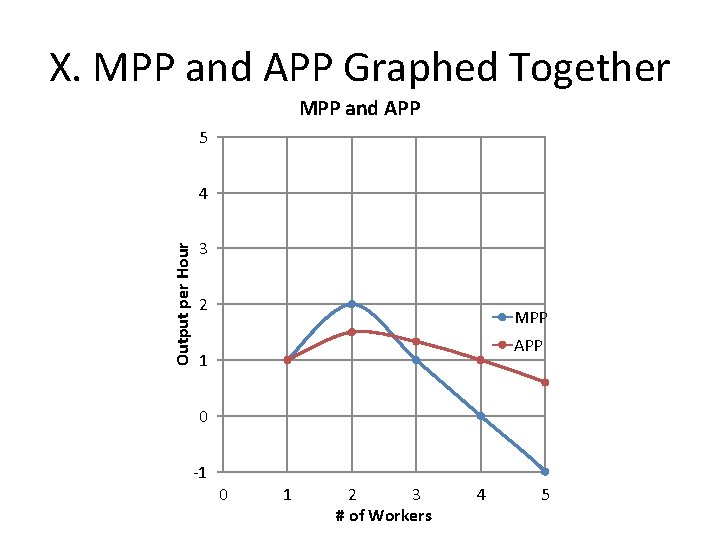
X. MPP and APP Graphed Together MPP and APP 5 Output per Hour 4 3 2 MPP APP 1 0 -1 0 1 2 3 # of Workers 4 5

XI. Where to Produce (so far)? • Based on what we know so far, where would you want to produce? – Maximize TPP? • no, the goal of firms is not to produce as much as possible – Maximize MPP? • no, would you want to maximize your marginal GPA if a lower GPA could still pull up your average GPA?

– Maximize Average APP? • yes, because you are maximizing the productivity of your labor…the units per worker is the highest – 1 worker can produce 1 unit for an average of 1 unit per worker, but 2 workers can produce 3 units for an average of 1. 5 units per worker • which means that the labor cost per unit is the lowest – at a production level of 1 unit, it requires an entire worker’s hour per unit (1 worker/1 unit), but producing 3 units requires only. 67 of a worker’s hour per unit (2 workers/3 units) – we only have to pay. 67 of an hour’s wages per unit when we produce 3 units instead of an entire hour’s wages when we produce 1 unit • we are minimizing our average labor cost per unit • but there are other costs to consider besides labor…which is tomorrow’s concept!!!

Upward Slope of the Supply Curve II: Costs of Production Unit 7: Producers and Supply

I. Translating Physical Product into Costs • as output rises, costs obviously rise, but how? • yesterday we looked at the relationship between workers and productivity (output or physical product) • today we will look at the relationship between productivity and costs

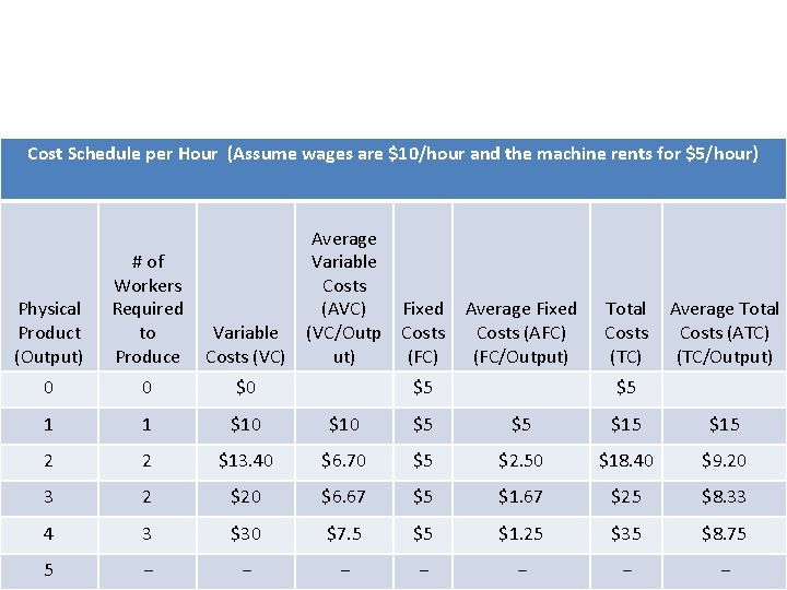
Cost Schedule per Hour (Assume wages are $10/hour and the machine rents for $5/hour) Average Variable Costs (AVC) Fixed (VC/Outp Costs ut) (FC) Physical Product (Output) # of Workers Required to Produce Variable Costs (VC) 0 0 $0 1 1 $10 $5 $5 $15 2 2 $13. 40 $6. 70 $5 $2. 50 $18. 40 $9. 20 3 2 $20 $6. 67 $5 $1. 67 $25 $8. 33 4 3 $30 $7. 5 $5 $1. 25 $35 $8. 75 5 − − − − Average Fixed Costs (AFC) (FC/Output) $5 Total Costs (TC) Average Total Costs (ATC) (TC/Output) $5

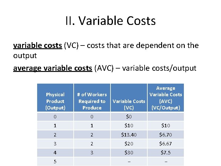
II. Variable Costs variable costs (VC) – costs that are dependent on the output average variable costs (AVC) – variable costs/output Average Variable Costs (AVC) (VC/Output) Physical Product (Output) # of Workers Required to Produce 0 0 $0 1 1 $10 2 2 $13. 40 $6. 70 3 2 $20 $6. 67 4 3 $30 $7. 5 − − 5

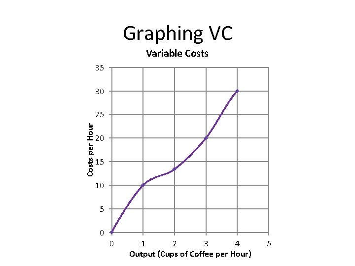
Graphing VC Variable Costs 35 30 Costs per Hour 25 20 15 10 5 0 0 1 2 3 4 Output (Cups of Coffee per Hour) 5

How does VC Change? • rises rapidly at first when we go from producing nothing to one • then rises at a decreasing rate because we become more productive with the next units we produce • then rises at an increasing rate because we become less productive with every unit we produce thereafter

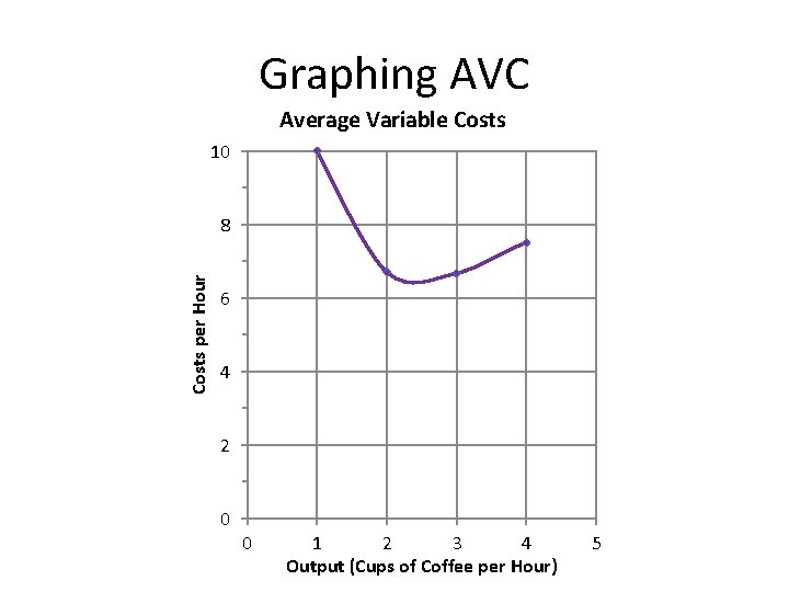
Graphing AVC Average Variable Costs 10 Costs per Hour 8 6 4 2 0 0 1 2 3 4 Output (Cups of Coffee per Hour) 5

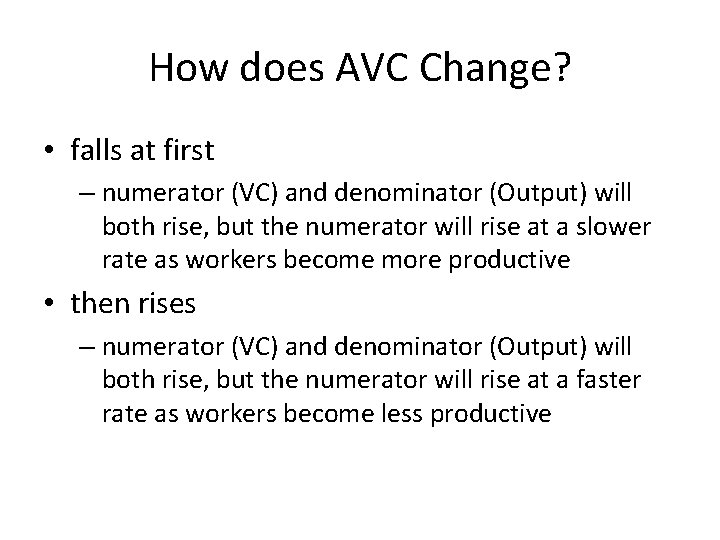
How does AVC Change? • falls at first – numerator (VC) and denominator (Output) will both rise, but the numerator will rise at a slower rate as workers become more productive • then rises – numerator (VC) and denominator (Output) will both rise, but the numerator will rise at a faster rate as workers become less productive

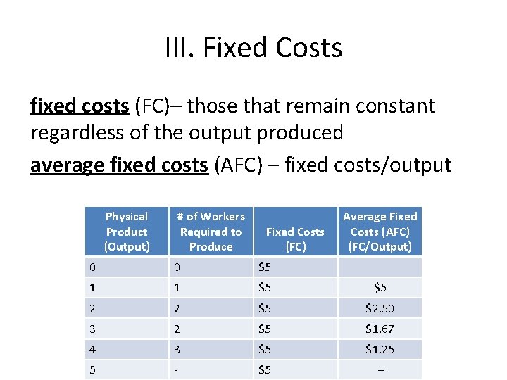
III. Fixed Costs fixed costs (FC)– those that remain constant regardless of the output produced average fixed costs (AFC) – fixed costs/output Physical Product (Output) # of Workers Required to Produce Fixed Costs (FC) Average Fixed Costs (AFC) (FC/Output) 0 0 $5 1 1 $5 $5 2 2 $5 $2. 50 3 2 $5 $1. 67 4 3 $5 $1. 25 5 - $5 −

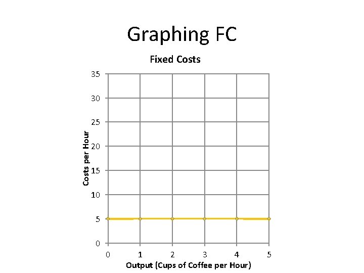
Graphing FC Fixed Costs 35 30 Costs per Hour 25 20 15 10 5 0 0 1 2 3 4 Output (Cups of Coffee per Hour) 5

How does FC Change? • they don’t…they are constant whether we produce 0 or 5

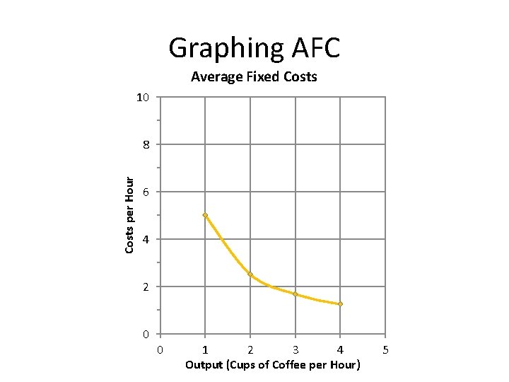
Graphing AFC Average Fixed Costs 10 Costs per Hour 8 6 4 2 0 0 1 2 3 4 Output (Cups of Coffee per Hour) 5

How does AFC Change? • falls at a decreasing rate – numerator is (FC) is constant, and denominator (Output) is always rising, but by a smaller and percentage (from 1 to 2 to 3 to 4, etc. )

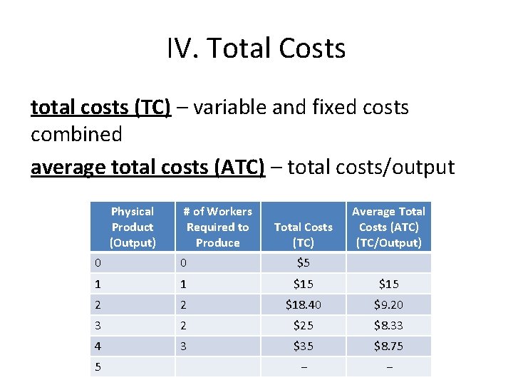
IV. Total Costs total costs (TC) – variable and fixed costs combined average total costs (ATC) – total costs/output Physical Product (Output) # of Workers Required to Produce Total Costs (TC) Average Total Costs (ATC) (TC/Output) 0 0 $5 1 1 $15 2 2 $18. 40 $9. 20 3 2 $25 $8. 33 4 3 $35 $8. 75 − − 5

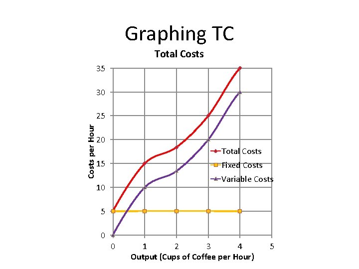
Graphing TC Total Costs 35 30 Costs per Hour 25 20 Total Costs 15 Fixed Costs Variable Costs 10 5 0 0 1 2 3 4 Output (Cups of Coffee per Hour) 5

How does TC Change? • since it is dependent on Variable Costs, it will mirror the Variable Cost Curve: – rises rapidly at first when we go from producing nothing to one – then rises at a decreasing rate because we become more productive with the next units we produce – then rises at an increasing rate because we become less productive with every unit we produce thereafter

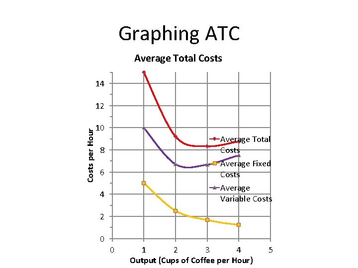
Graphing ATC Average Total Costs 14 Costs per Hour 12 10 8 Average Total Costs 6 Average Fixed Costs 4 Average Variable Costs 2 0 0 1 2 3 4 Output (Cups of Coffee per Hour) 5

How does ATC Change? • falls at first because AFC and AVC are both falling • then rises when the rise of AVC offsets the fall in AFC (which is falling at a decreasing rate…its flattening out)

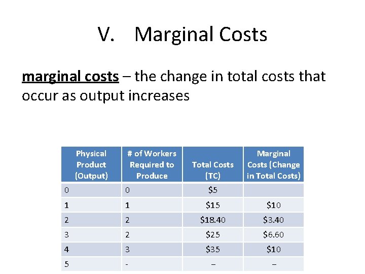
V. Marginal Costs marginal costs – the change in total costs that occur as output increases Physical Product (Output) # of Workers Required to Produce Total Costs (TC) Marginal Costs (Change in Total Costs) 0 0 $5 1 1 $15 $10 2 2 $18. 40 $3. 40 3 2 $25 $6. 60 4 3 $35 $10 5 - − −

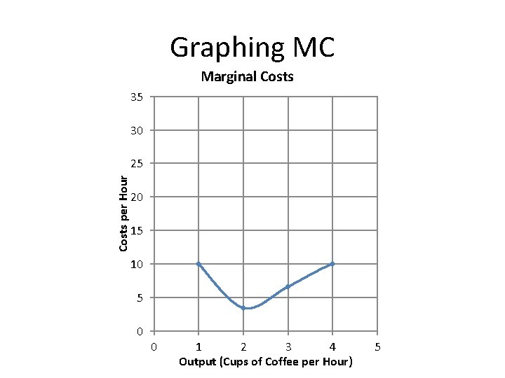
Graphing MC Marginal Costs 35 30 Costs per Hour 25 20 15 10 5 0 0 1 2 3 4 Output (Cups of Coffee per Hour) 5

How does MC Change? • falls at first with the first couple units of output as we become more productive • then begins to rise as we become less and less productive the more units of output we produce

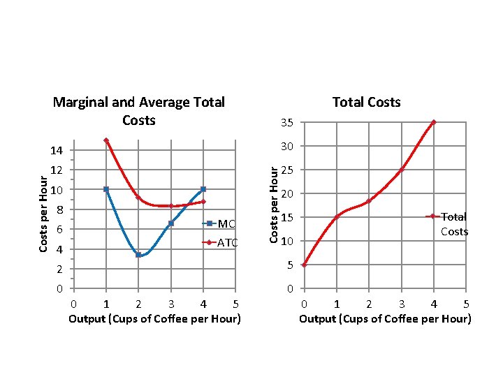
VI. What do we Need to Know? 1. 2. 3. out of all this, we need to understand the shape of the ATC curve and the MC curve (U-shaped) we need to understand why they’re shaped that way (law of diminishing marginal product) we need to understand how they are related to each other

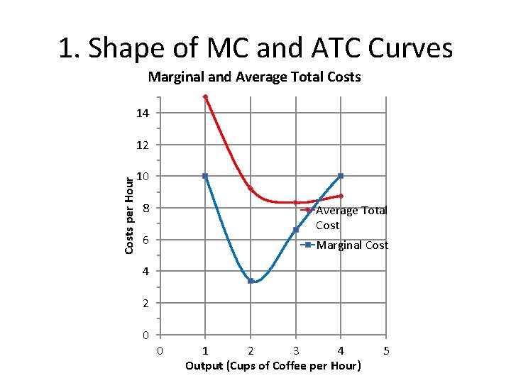
1. Shape of MC and ATC Curves Marginal and Average Total Costs 14 Costs per Hour 12 10 8 Average Total Cost 6 Marginal Cost 4 2 0 0 1 2 3 4 Output (Cups of Coffee per Hour) 5

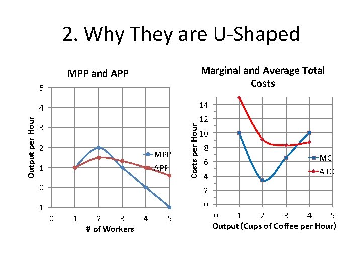
2. Why They are U-Shaped 5 Marginal and Average Total Costs 4 14 3 2 MPP 1 APP Costs per Hour Output per Hour MPP and APP 12 10 8 6 4 0 2 -1 0 0 1 2 3 # of Workers 4 5 MC ATC 0 1 2 3 4 5 Output (Cups of Coffee per Hour)

• they are U-shaped because the MPP and APP curves are hump shaped • as productivity per worker (MPP and APP) rises then falls, costs per unit (MC and ATC) will fall then rise

3. How are MC and ATC Related? • just like the relationship between MPP and APP (and marginal and average GPA), MC and ATC are directly related • if MC is below ATC, it will pull down ATC • if MC is above ATC is will pull up ATC • MC will always intersects ATC at its minimum point

VII. Where do we want to produce at (so far)? • do we care about variable or fixed? – no, we care about total • do we want to minimize total costs? – no, then we would produce zero • do we want to minimize MC? – no, just like we didn’t want to maximize MPP • do we want to minimize ATC? – yes, just like we wanted to maximize APP – in fact, they are related, if this is where we are maximizing productivity, this is where we are minimizing cost per unit (ATC) – but, that’s only one part of the profit equation (costs)…what about revenue…tomorrow’s lesson

The Upward Slope of the Supply Curve III: Revenue and Profit Maximization Unit 7: Producers and Supply

I. The Perfectly Competitive Firm’s Demand Curve • it is perfectly elastic • perfectly competitive firms are price takers…they take the market price – remember • large # of firms • standardized products • easy entry • they can’t raise the price because demand will be zero and they won’t lower price because they will lose money

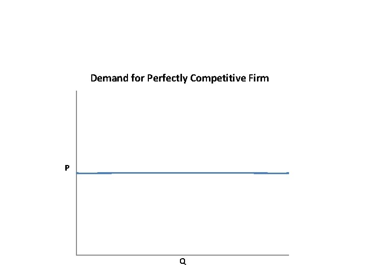
Demand for Perfectly Competitive Firm P Q

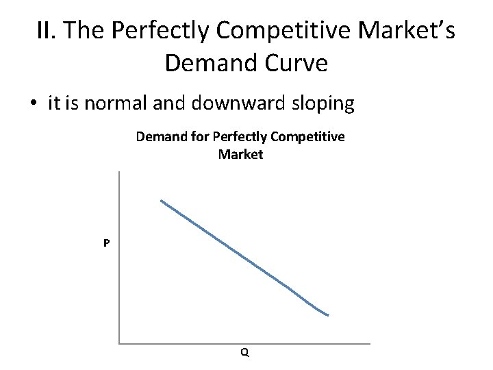
II. The Perfectly Competitive Market’s Demand Curve • it is normal and downward sloping Demand for Perfectly Competitive Market P Q

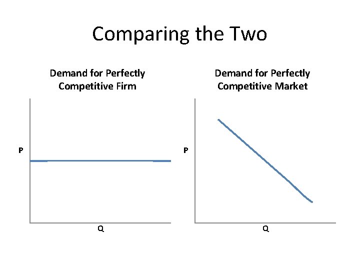
Comparing the Two Demand for Perfectly Competitive Firm P Demand for Perfectly Competitive Market P Q Q

III. Review of Costs • we’ll come back to the perfectly elastic demand curve for a perfectly competitive firm in a little bit • remember the goal of producers is to maximize total profit (TP = TR – TC) • yesterday we saw how costs change as we produce more output • obviously total costs (TC) will rise, first at a decreasing then increasing rate, because marginal costs (MC) and average total costs (ATC)…costs per unit…will fall then rise according to the law of diminishing marginal product • first we become more productive, then we become less productive • if we want to minimize costs per unit, we would produce at minimum ATC • but that’s only one variable in the profit equation (costs)…what about revenue?

35 14 30 12 25 10 8 6 4 MC ATC Total Costs per Hour Marginal and Average Total Costs 20 15 10 2 5 0 0 0 1 2 3 4 5 Output (Cups of Coffee per Hour) Total Costs 0 1 2 3 4 5 Output (Cups of Coffee per Hour)

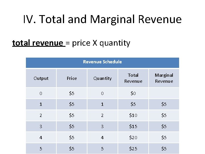
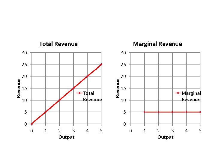
IV. Total and Marginal Revenue total revenue = price X quantity Revenue Schedule Output Price Quantity Total Revenue Marginal Revenue 0 $5 0 $0 1 $5 $5 2 $10 $5 3 $15 $5 4 $20 $5 5 $25 $5

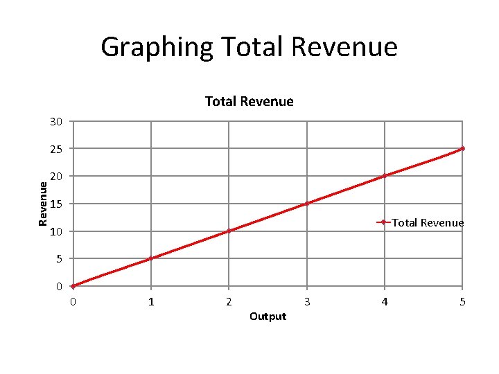
Graphing Total Revenue 30 Revenue 25 20 15 Total Revenue 10 5 0 0 1 2 Output 3 4 5

How does TR change? • it will rise at a constant rate • the price of the product does not change • every unit we produce (and sell) will cause TR to go up by that constant price of the product

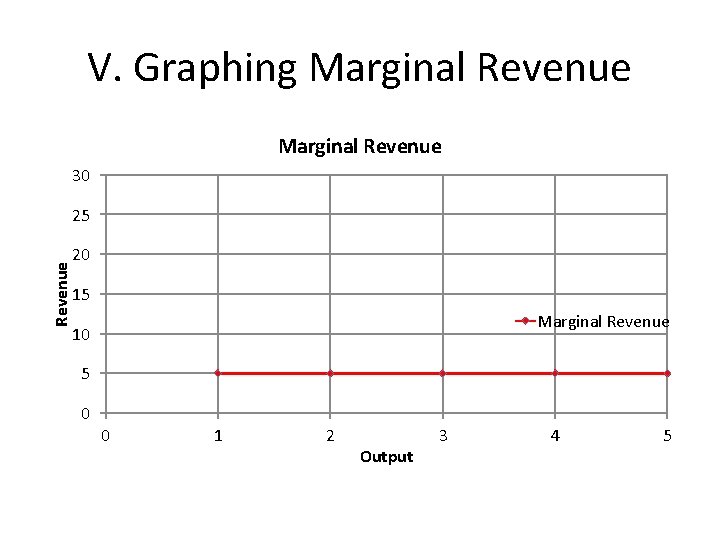
V. Graphing Marginal Revenue 30 Revenue 25 20 15 Marginal Revenue 10 5 0 0 1 2 Output 3 4 5

How does MR Change? • it is constant…the price of the product • every unit we produce (and sell) will cause TR to go up by that constant price of the product

Marginal Revenue 30 30 25 25 20 20 15 Total Revenue 10 Revenue Total Revenue 15 10 5 5 0 0 0 1 2 3 Output 4 5 Marginal Revenue 0 1 2 3 Output 4 5

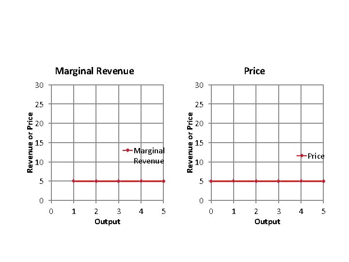
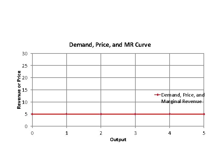
VI. MR = Price • in a perfectly competitive market, MR = P • the revenue brought in by each unit we sell is simply the price of that product • since the price doesn’t change the more we produce, the MR will not change – in a perfectly competitive market, each producer is so small that their supply does not effect the market price

Price 30 30 25 25 20 15 Marginal Revenue 10 Revenue or Price Marginal Revenue 20 15 5 5 0 0 0 1 2 3 Output 4 5 Price 10 0 1 2 3 Output 4 5

VII. MR = Price = Demand • the demand curve for a perfectly competitive firm is a horizontal line at the market price • at the market price, consumers will demand as little or as much as they want from that firm • so regardless of the quantity supplied by the firm, the price of the product and therefore the marginal revenue will be the same

Demand, Price, and MR Curve 30 Revenue or Price 25 20 15 Demand, Price, and Marginal Revenue 10 5 0 0 1 2 Output 3 4 5

VIII. Maximizing Total Profit • the rule to maximize TP is ALWAYS the same: – produce until MC = MR – this makes sense…as long as the revenue brought in by one more unit of a good is greater than the cost of producing that good, it will add to our total profit – at any given quantity of output, if MR > MC, producing more will add to the total profit (or lessen the loss) – at any given quantity of output, if MR < MC, producing more will take away from total profit (or add to the total loss)

Maximizing Total Profit (P>ATC) Costs, Price, and Revenue per Unit Output

• produce until MC = MR • follow that quantity up to the ATC curve and trace it over to the y axis. . . this is your cost per unit at that quantity of output (ATC X Q = TC) • now, follow it up to price or demand curve and trace it over to the y -axis…this is your revenue per unit at that quantity of output (P X Q = TR • subtracting costs from revenue gives your total profit (TP = TR – TC) • if at that quantity where MR = MC, P > ATC, you will make a profit • if at that quantity where MR = MC, P = ATC, you will breakeven • if at that quantity where MR =MC, P < ATC, you will lose money, but you will minimize your loss at that point, you can do no better

Breakeven (P=ATC) Costs, Price, and Revenue per Unit Output

Loss Minimization (P<ATC) Costs, Price, and Revenue per Unit Output

Why don’t we want to minimize ATC? • producing at minimum ATC will maximize average profit, but we want to maximize total profit! • continuing to produce until MC = MR will cause average profit to decrease, but as long as we’re still making a profit on each unit we produce (even if it’s smaller and smaller) it will still add to our total profit • maximizing total height example

Average Profit vs. Total Profit Costs, Price, and Revenue per Unit Output

Upward Slope of the Supply Curve IV: The Short-and Long-run Shutdown Decisions and Supply Curves Unit 7: Producers and Supply

I. Review: Shape of the Supply Curve • firms will always maximize total profit or minimize total loss by producing where MC=MR • this quantity depends on P (MR=P) • ↑ P means ↑ Q that will maximize total profit • ↓ P means ↓ Q that will maximize total profit • basically higher prices mean firms will make a greater profit on each unit and will continue to make a marginal profit on more units than lower prices • this is the reason for the upward slope of the supply curve

• if at the profit maximizing quantity: § P > ATC = Profit § P = ATC = Breakeven § P < ATC = Loss • since we always produce where MC = MR, and since MR = P, then we always produce where MC = P (or where the MC curve intersects the P curve) • the MC curve is the firm’s supply curve!!!

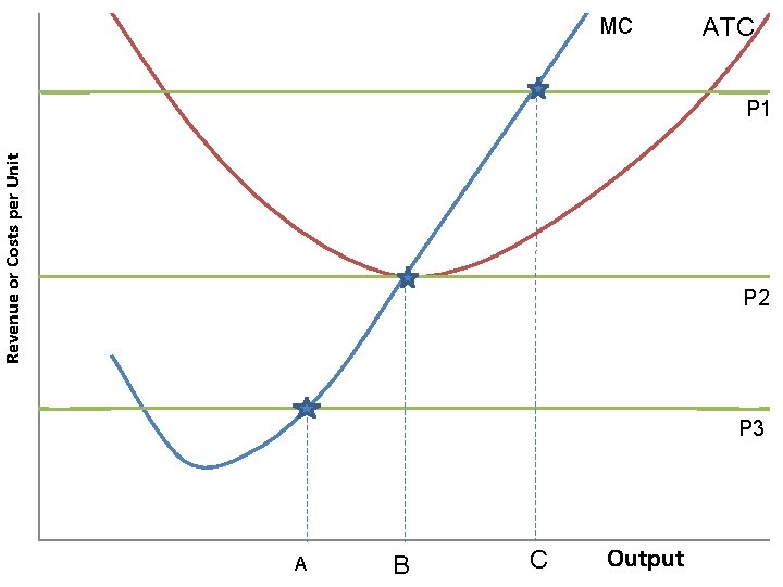
Revenue or Costs per Unit MC A B C Output ATC P 1 P 2 P 3

II. Why Would a Firm Operate at a Loss? • if prices are low enough, the best a firm could do is minimize it’s loss, in other words it can’t earn a profit at that price • why would a firm do this?

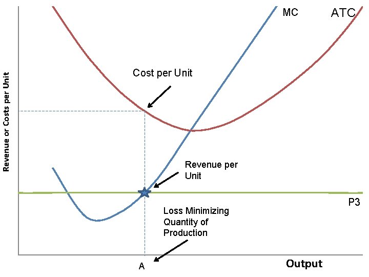
Revenue or Costs per Unit MC ATC Cost per Unit Revenue per Unit P 3 Loss Minimizing Quantity of Production A Output

• it might actually be cheaper for a firm to operate at a loss in the short-run than to shutdown • remember, even if a firm produces nothing, it still has fixed costs • if the price of the product is high enough to at least cover it’s variable costs, then it can use any left over to at least pay some of its fixed costs

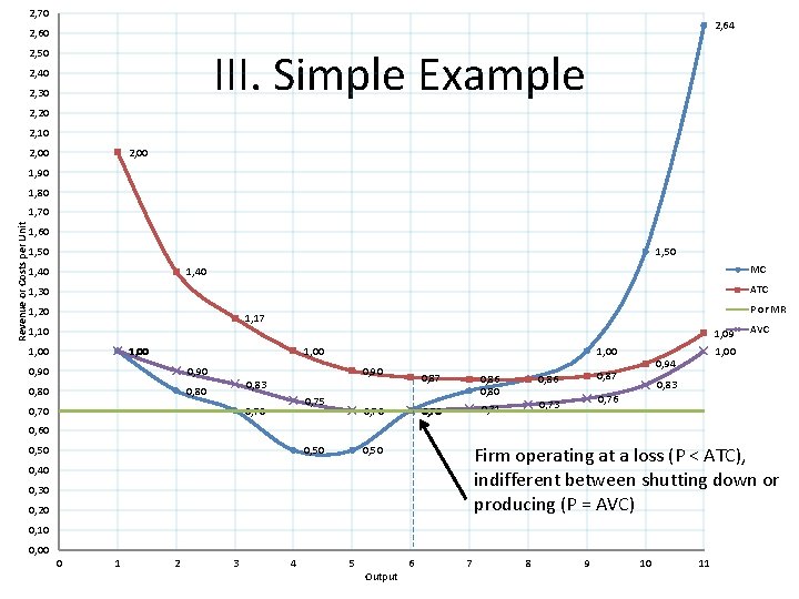
2, 70 2, 64 2, 60 III. Simple Example 2, 50 2, 40 2, 30 2, 20 2, 10 2, 00 1, 90 1, 80 Revenue or Costs per Unit 1, 70 1, 60 1, 50 1, 40 MC 1, 40 ATC 1, 30 1, 20 P or MR 1, 17 1, 10 1, 09 1, 00 0, 90 0, 80 1, 00 0, 90 0, 83 0, 70 0, 75 0, 70 0, 87 0, 70 0, 86 0, 80 0, 86 0, 71 0, 73 1, 00 0, 94 0, 87 AVC 0, 83 0, 76 0, 60 0, 50 Firm operating at a loss (P < ATC), indifferent between shutting down or producing (P = AVC) 0, 50 0, 40 0, 30 0, 20 0, 10 0, 00 0 1 2 3 4 5 Output 6 7 8 9 10 11

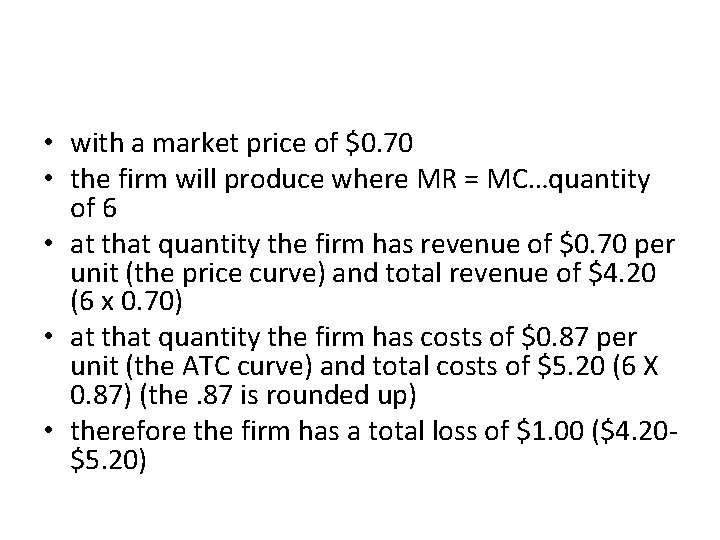
• with a market price of $0. 70 • the firm will produce where MR = MC…quantity of 6 • at that quantity the firm has revenue of $0. 70 per unit (the price curve) and total revenue of $4. 20 (6 x 0. 70) • at that quantity the firm has costs of $0. 87 per unit (the ATC curve) and total costs of $5. 20 (6 X 0. 87) (the. 87 is rounded up) • therefore the firm has a total loss of $1. 00 ($4. 20$5. 20)

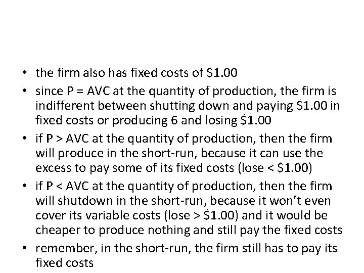
• the firm also has fixed costs of $1. 00 • since P = AVC at the quantity of production, the firm is indifferent between shutting down and paying $1. 00 in fixed costs or producing 6 and losing $1. 00 • if P > AVC at the quantity of production, then the firm will produce in the short-run, because it can use the excess to pay some of its fixed costs (lose < $1. 00) • if P < AVC at the quantity of production, then the firm will shutdown in the short-run, because it won’t even cover its variable costs (lose > $1. 00) and it would be cheaper to produce nothing and still pay the fixed costs • remember, in the short-run, the firm still has to pay its fixed costs

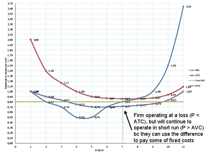
2, 70 2, 64 2, 60 2, 50 2, 40 2, 30 2, 20 2, 10 2, 00 1, 90 1, 80 Revenue or Costs per Unit 1, 70 1, 60 1, 50 1, 40 MC 1, 40 ATC 1, 30 1, 20 P or MR 1, 17 1, 10 1, 09 1, 00 0, 90 0, 80 1, 00 0, 90 0, 83 0, 70 0, 75 0, 70 0, 87 0, 70 0, 60 0, 50 0, 30 0, 20 0, 10 0, 00 1 2 3 4 5 Output 0, 86 0, 71 0, 73 1, 00 0, 94 0, 87 0, 83 0, 76 Firm operating at a loss (P < ATC), but will continue to operate in short run (P > AVC) bc they can use the difference to pay some of fixed costs 0, 50 0, 40 0 0, 86 0, 80 AVC 6 7 8 9 10 11

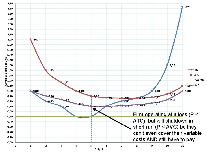
2, 70 2, 64 2, 60 2, 50 2, 40 2, 30 2, 20 2, 10 2, 00 1, 90 1, 80 Revenue or Costs per Unit 1, 70 1, 60 1, 50 1, 40 MC 1, 40 ATC 1, 30 1, 20 P or MR 1, 17 1, 10 1, 09 1, 00 0, 90 0, 80 1, 00 0, 90 0, 83 0, 70 0, 75 0, 70 0, 87 0, 70 0, 60 0, 50 0, 30 0, 20 0, 10 0, 00 1 2 3 4 5 Output 0, 86 0, 71 0, 73 1, 00 0, 94 0, 87 0, 83 0, 76 Firm operating at a loss (P < ATC), but will shutdown in short run (P < AVC) bc they can’t even cover their variable costs AND still have to pay 0, 50 0, 40 0 0, 86 0, 80 AVC 6 7 8 9 10 11

IV. Short-run Shutdown Decision • in the short-run, as long as the firm expects the future to be better, the firm will continue to operate at a loss as long as P = or > AVC (cheaper than completely shutting down) • in the short-run, the firm will shutdown if P < AVC (cheaper to just shutdown)

V. Long-run Shutdown Decision • in the long-run, the firm can shutdown completely and avoid paying fixed costs (sell factory, machines, etc. ) • in the long run, the firm will continue to operate if P > or = ATC • in the long-run the firm will shutdown if P < ATC

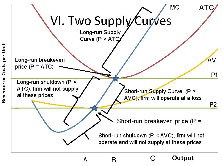
Revenue or Costs per Unit MC ATC VI. Two Supply Curves Long-run Supply Curve (P > ATC) Long-run breakeven price (P = ATC) AV P 1 Long-run shutdown (P < ATC), firm will not supply at these prices Short-run Supply Curve (P > AVC), firm will operate at a loss P 2 Short-run breakeven price (P = Short-run shutdown (P < AVC), firm will not operate and will not supply at these prices A B C Output

• there are essentially two supply curves: – short-run: portion of MC curve between AVC and ATC – long-run: portion of MC curve above the ATC curve

Economies of Scale Unit 7: Producers and Supply

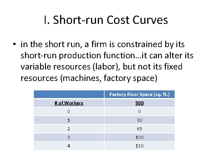
I. Short-run Cost Curves • in the short run, a firm is constrained by its short-run production function…it can alter its variable resources (labor), but not its fixed resources (machines, factory space) Factory Floor Space (sq. ft. ) # of Workers 500 0 0 1 30 2 65 3 100 4 130

• the productivity that is reflected in this production function is also reflected in its short-run cost curves • once the firm has selected its factory size, it’s in the short-run and its cost per unit is reflected by the short-run ATC curve • it can alter its output anywhere along that ATC curve

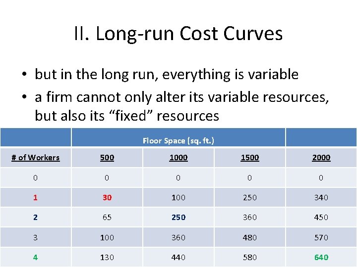
II. Long-run Cost Curves • but in the long run, everything is variable • a firm cannot only alter its variable resources, but also its “fixed” resources Floor Space (sq. ft. ) # of Workers 500 1000 1500 2000 0 0 1 30 100 250 340 2 65 250 360 450 3 100 360 480 570 4 130 440 580 640

• notice that as we double the size of the firm (from 1 to 2 employees and from 500 sq. ft. to 1000 sq. ft. ) we are doubling our costs, but more than doubling our output (from 30 to 250) • this happens again as we go from 2 to 4 employees and from 1, 000 sq. ft. to 2, 000 sq. ft. • this means we are getting more productive as we get bigger, which means the cost per unit (ATC) goes down as we get bigger and produce more

• the productivity that is reflected in this production function is reflected in the lower SRATC curves for each different scale (size) of the firm • each SRATC curve represents the costs per unit for any given factory size • once a firm selects its factory size, it is in the short-run and can only operate along that particular SRATC • but in the long-run, a firm can select any factory size and operate along any of the SRATC curves

III. Economies of Scale economies of scale – the increase in productivity and corresponding decrease in per unit cost (ATC) as firms grow in size when all resources are variable in the long run

IV. Long-run Average Total Cost (LRATC) Curve • connects the lowest cost per unit (ATC) possible for every unit of production when all resources are variable • it just touches each SRATC curve • in the long-run, a manager can produce whatever quantity they want and then choose the least-cost combination of resources to produce that (a point on the LRATC)

• if a firm is operating along SRATC 2 in the shortrun and produces at Q 1 it will have costs at Point A (not on the LRATC) • in the long-run, the manager will logically add more fixed resources, move to SRATC 3, produce at Q 1, but only have costs at Point B (on the LRATC)

• this will continue until the firm reaches the minimum efficient scale • minimum efficient scale (MES) – the minimum point of the LRATC curve • this is the most productive size for the firm and the cheapest per unit cost that can possibly be achieved • after this, the larger the firm gets , the less productive it becomes, the higher the cost per unit (ATC), and diseconomies of scale kick in

diseconomies of scale – when a firm increases in size, but its productivity does not increase proportionally (doubles its size and costs, but does not double its output)

• if a firm is operating along SRATC 6 in the shortrun and is producing at Q 2 it will have costs at Point C • but in the long-run, the firm will sell off parts of its business or resources, move to SRATC 5, produce at Q 2 and have costs at Point D