Supply Chain Modeling Language SCML Project Mikio KUBO
 Project Mikio KUBO Tokyo University of Marine Science of")
Supply Chain Modeling Language (SCML) Project Mikio KUBO Tokyo University of Marine Science of Technology http: //kubomikio. com

Koji Nonobe @ Hosei University Mutsunori Yagiura @Nagoya University Hideki Hashimoto @Nagoya University J. Pedroso @ Porto University

What is the SCML? Solvers Supply Chain Optimization Models Combinatorial Optimization Problems SCML AMPL Model Files
, lot-sizing (LS) logistics network")
Supply chain optimization models • • resource constrained scheduling (RCS), lot-sizing (LS) logistics network design (LND) safety stock allocation (SSA) economic order quantity (EOQ) inventory policy optimization (IPO) vehicle routing (VR)
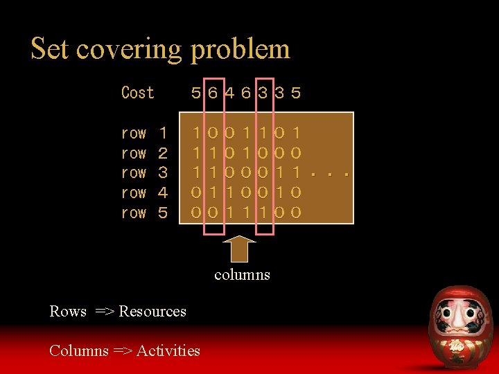
 set covering problem (SCP)")
Combinatorial optimization problems • • • generalized assignment problem (GAP) set covering problem (SCP) rectangular packing problem (RPP) multi-dimensional knapsack problem (MKP) facility location problem (FLP)
 model • SCML (same name!) :")
Related work • SCOR (supply chain operations reference) model • SCML (same name!) : supply chain modeling language for simulation • Algebraic modeling languages

SCOR model proposed by Supply Chain Council A reference model designed for effective communication among SC partners SC= {(plan, source, make deliver, return). . . }
 XML-based document format for simulation Basic entities are:")
Another SCML Chatfield et al. (2009) XML-based document format for simulation Basic entities are: • node and arc (network is essential) • component (≒ product + resource) • action (≒ activity) • policy (for doing simulation)
 –")
Algebraic modeling languages • AMPL, MOSEL, OPL, GAMS, etc. • solvers (general purpose) – Mixed integer programming, constrained programming, other nonlinear programming • using set, parameter, variable, objective function, constraints, etc. (also general purpose)

Previous work • Activity based view of linear programming Resource constrained scheduling model • Lot-sizing models • State-task network representation for batch process • Logistics network design model • Algebraic modeling languages
![Activity based view of linear programming Dantzig-Wolfe (1963) matrix A=[aij] row =resource + +](http://slidetodoc.com/presentation_image_h/08197ac59d62ec9f9de9a41fb62125f3/image-11.jpg "Activity based view of linear programming Dantzig-Wolfe (1963) matrix A=[aij] row =resource + +")
Activity based view of linear programming Dantzig-Wolfe (1963) matrix A=[aij] row =resource + + b - activity i consumes resource j by aij column =activity (amount: Xj) system input of resource

Resource constrained scheduling model activity require resource precedence relation
 resource product")
Lot-sizing models BOM (bill of material) resource product
 task =activity resource state = product")
State-task network representation Kandili-Pantelides-Sargent (1993) task =activity resource state = product

Logistics network design model node resource node require assemble disassemble product transport

Key entities • • activity resource product node arc horizon mode state, temporal, piecewise, solver …

Activity • Every action that requires the resources, consumes and/or produces the product, and derives the cost consume product Fixed Cost Variable Cost activity require resource product

Resource • Every entity of limited availability Our focus is on the physical, human, and financial resources. • Categorized into: – Renewable – Nonrenewable

Product , node, arc • A product is an item or commodity through the network • Network is defined by the set of nodes and arcs node product arc node product

Relation among entities arc node consume product produce activity product require resource Activities and resources can be defined on arcs. (They are called “local. ” Otherwise called “global. ”) Products are defined on nodes.

Notations • • • inf : ∞ integer+: a non-negative integer or +∞ integer: an integer or +∞ or -∞ real+: a non-negative real number or +∞ real: a real number or +∞ or -∞ range: a pair of two integers (a, b) such that a ≦ b. . . : allow any number of repetitions [ ] : optional { } : select one within the braces

Horizon horizon declaration: horizon integer+ horizon 4 0 1 2 3 4 set the planning horizon to 4
![Activity attributes [autoselect] mode-name. . . mode [mode-attributes] duedate integer+ weight integer+ start {](http://slidetodoc.com/presentation_image_h/08197ac59d62ec9f9de9a41fb62125f3/image-23.jpg "Activity attributes [autoselect] mode-name. . . mode [mode-attributes] duedate integer+ weight integer+ start {")
Activity attributes [autoselect] mode-name. . . mode [mode-attributes] duedate integer+ weight integer+ start { integer+, range, piecewise-name } completion { integer+, range, piecewise-name } selected { mode-name, resource-name} execute interval range [parallel integer+]. . .
 3 4")
Interval 0 1 2 interval 1 3 => {②, ③} [1, 3) 3 4 ①②③④ range execute interval 1 3 execute interval 3 4 parallel 2 0 1 2 3 4
![Mode attributes duration integer+ resource-name [max] [ interval range] requirement integer+ cost { integer,](http://slidetodoc.com/presentation_image_h/08197ac59d62ec9f9de9a41fb62125f3/image-25.jpg "Mode attributes duration integer+ resource-name [max] [ interval range] requirement integer+ cost { integer,")
Mode attributes duration integer+ resource-name [max] [ interval range] requirement integer+ cost { integer, piecewise-name }. . . break interval range [max] integer+. . . parallel interval range [max] integer+. . . state-name from state-value to state-value amount interval range real+ (LS, LND) consume product-name unit real+. . . produce product-name unit real+. . . variablecost [interval range] real. . . fixedcost [interval range] real. . . cycletime [interval range] { integer+, range } leadtime [ interval range] { integer+, range }
![Resource attributes [interval range] capacity integer+. . . location node-name time integer+ cost real](http://slidetodoc.com/presentation_image_h/08197ac59d62ec9f9de9a41fb62125f3/image-26.jpg "Resource attributes [interval range] capacity integer+. . . location node-name time integer+ cost real")
Resource attributes [interval range] capacity integer+. . . location node-name time integer+ cost real interval 0 1 capacity 1 interval 1 3 capacity 2 interval 3 4 capacity 1 0 1 2 3 4
![Temporal constraints temporal declaration: temporal activity-name [attributes] attribute: type { SS, SC, CS, CC](http://slidetodoc.com/presentation_image_h/08197ac59d62ec9f9de9a41fb62125f3/image-27.jpg "Temporal constraints temporal declaration: temporal activity-name [attributes] attribute: type { SS, SC, CS, CC")
Temporal constraints temporal declaration: temporal activity-name [attributes] attribute: type { SS, SC, CS, CC } delay integer Completion Start delay A B

States state declaration: state-name time integer+ value integer+. . .

Piecewise linear function attributes interval range init real slope real. . . default real piecewise example default inf interval 0 1 init 1 slope 1 interval 1 3 init 1 slope 0 Must be lower semicontinous
![Product attributes supply [interval range] {real+, range, randvar }. . . demand [interval range]](http://slidetodoc.com/presentation_image_h/08197ac59d62ec9f9de9a41fb62125f3/image-30.jpg "Product attributes supply [interval range] {real+, range, randvar }. . . demand [interval range]")
Product attributes supply [interval range] {real+, range, randvar }. . . demand [interval range] {real+, range, randvar }. . . holdingcost [interval range] real+. . . backordercost [interval range] real+. . . inventory [interval range] real+. . . capacity [interval range] real+. . . variability real+ safetyratio real+ reorderpoint real+ basestocklevel real+
![Nodes node declaration: node-name [attributes] attribute: location latitude longitude weight real+ product-name [product-attributes]. .](http://slidetodoc.com/presentation_image_h/08197ac59d62ec9f9de9a41fb62125f3/image-31.jpg "Nodes node declaration: node-name [attributes] attribute: location latitude longitude weight real+ product-name [product-attributes]. .")
Nodes node declaration: node-name [attributes] attribute: location latitude longitude weight real+ product-name [product-attributes]. . .
![Arcs arc-name node-name [attributes] attribute: cost real time { real+, piecewise-name } distance real+](http://slidetodoc.com/presentation_image_h/08197ac59d62ec9f9de9a41fb62125f3/image-32.jpg "Arcs arc-name node-name [attributes] attribute: cost real time { real+, piecewise-name } distance real+")
Arcs arc-name node-name [attributes] attribute: cost real time { real+, piecewise-name } distance real+ activity-name [activity-attributes]. . . resource-name [resource-attributes]. . .

Solvers solver declaration: solver { RCS, LND, SSA, EOQ, IPO, VR, SCP, GAP, RPP, MKP, FLP} [attributes] attribute: option-name option-value. . .
 attributes : children activity (resource, product)-name. . . [type {")
Hierarchies activity (resource, product) attributes : children activity (resource, product)-name. . . [type { and, or } ] Modes: children of an activity with type “or” Vehicle capacities (weight, volume, . . . ) : children of a resource (vehicle) with type “and”
![Scheduling model • [horizon], activity, mode, resource, nonrenewable, temporal, state temporal activity state require](http://slidetodoc.com/presentation_image_h/08197ac59d62ec9f9de9a41fb62125f3/image-35.jpg "Scheduling model • [horizon], activity, mode, resource, nonrenewable, temporal, state temporal activity state require")
Scheduling model • [horizon], activity, mode, resource, nonrenewable, temporal, state temporal activity state require modes resource require nonrenewable
 resource writer activity B duedate 9 weight 5 interval 0 3")
Scheduling model (example) resource writer activity B duedate 9 weight 5 interval 0 3 capacity 1 mode duration 2 interval 4 6 capacity 1 writer interval 0 2 requirement 1 interval 7 10 capacity 1 break interval 0 2 max 1 interval 11 inf capacity 1 activity A duedate 5 weight 20 mode duration 1 writer interval 0 1 requirement 1 . . . solver RCS option time 100

Lot-sizing model • horizon, activity, mode, resource, product consume activity resource product produce
 : G=(N, A) φpq: the units of product")
BOM • BOM (bill of materials) : G=(N, A) φpq: the units of product p to produce one unit of product q. p φpq child product of q product q resource parent product of q

BOM representation using SCML consume product activity produce child activity resource parent
 horizon 5 product prod 1 holdingcost 0 inf 5 demand interval")
Lot-sizing model (example) horizon 5 product prod 1 holdingcost 0 inf 5 demand interval 0 1 5 demand interval 1 2 7 demand interval 2 3 3 demand interval 3 4 6 demand interval 4 5 4 resource res 1 interval 0 inf capacity 25 activity act 1 mode duration 1 variablecost interval 0 inf 1 fixedcost interval 0 inf 53 #setup cost leadtime interval 0 inf 3 res 1 interval 0 inf requirement 1 consume parts 1 unit 1 product parts 1 holdingcost 0 inf 1. . . #setup time consume parts 2 unit 2 generate prod 1 unit 1 solver LS
 model • horizon, activity, resource, product, node, arc node consume")
Logistics network design (LND) model • horizon, activity, resource, product, node, arc node consume product activity produce require resource product

An example of LND model source 1 vehicle line 1 apple vehicle plantout plantin juice source 2 line 2 ship apple × 2 bottle customer juice
 1 horizon 2 product apple holdingcost 5 inf 5 product")
LND model (SCML example) 1 horizon 2 product apple holdingcost 5 inf 5 product bottle holdingcost 1 inf 5 product juice variability 1 safetyratio 1. 65 node source 1 apple supply interval 0 inf 100 node source 2 bottle supply interval 0 inf 100 node plantin node plantout juice holdingcost 10 node customer juice demand interval 0 inf 10 holdingcost 30
 2 arc source 1 plantin trans_apple #activity vehicle cost 10")
LND model (SCML example) 2 arc source 1 plantin trans_apple #activity vehicle cost 10 #resource arc source 2 plantin activity trans_apple mode duration 1 variablecost 0 inf 1 cycletime 0 inf 1 trans_bottle #activity vehicle requirement 1 ship cost 30 #resource consume apple unit 1 arc plantin plantout produce apple unit 1 prod_juice_online 1 activity trans_bottle prod_juice_online 2 mode duration 1 line 1 cost 50 variablecost 0 inf 1 line 2 cost 100 cycletime arc plantout customer 0 inf 1 ship requirement 1 trans_juice consume bottle unit 1 vehicle cost 20 produce bottle unit 1
 3 activity prod_juice_online 1 resource line 1 mode duration 1")
LND model (SCML example) 3 activity prod_juice_online 1 resource line 1 mode duration 1 interval 0 inf capacity 100 variablecost 0 inf 10 cost 70 cycletime 0 inf 5 resource line 2 line 1 requirement 1 interval 0 inf capacity 100 consume apple unit 2 cost 20 consume bottle unit 1 produce juice unit 1. . . resource vehicle interval 0 inf capacity 2 resource ship interval 0 inf capacity 10 solver LND

Vehicle routing model • activity, resource, node, arc, piecewise start piecewise completion piecewise “move” activity depot or origin vehicle resource weight resource volume resource a customer or destination
 economic ordering quantity model")
Inventory models • horizon, product, activity, resource • (network type) economic ordering quantity model (EOQ) • safety stock allocation model (SSA) • inventory policy optimization model (IPO)
 (EOQ) leadtime (range), cycletime (integer+), duration (SSA)")
Inventory models and BOM fixedcost, cycletime (range) (EOQ) leadtime (range), cycletime (integer+), duration (SSA) leadtime (integer+), cycletime (integer+) (IPO) activity resource product demand, holdingcost basestocklevel, backordercost (IPO) capacity (IPO)

Generalized assignment problem aij =>requirement bi =>capacity cij =>cost jobs => activities agents =>resources

Rectangular packing problem height =>resource rectangle =>activity with multiple modes cost => piecewise width =>resource

Multi-dimensional knapsack problem aij =>requirement bi profit pj => -cost items => activities =>capacity constraints =>resources

Other problems • facility location problem – defined on nodes: (x, y coordinates and weight) • traveling salesman problem – defined on nodes: (x, y coordinates) ; Euclidian TSP – defined on nodes and arcs (cost); general TSP • bin packing problem – defined on activities (items) and a resource (bin size)
- Slides: 53