Supply Chain Management Lecture 20 Outline Today Chapter

Supply Chain Management Lecture 20

Outline • Today – Chapter 11 • Sections 1, 2, 3, 7, 8 – Skipping 11. 2 “Evaluating Safety Inventory Given Desired Fill rate” • Thursday – Homework 4 due before class – Chapter 12 • Sections 12. 1, 12. 2 up to and including Example 12. 2, 12. 3 • Friday – Homework 5 online • Due Thursday April 8 before class

Staples Visit • Date – Friday April 2, 10: 30 am – 2: 30 pm • (11: 30 am – 1: 30 pm on site, the rest in transit) • Free transportation • Location – Staples fulfillment Center, Brighton, CO • What – Lunch and Learn Email: Ann. Richmond@colorado. edu

Summary • Inventory is an asset, but it's also a liability until it has been sold – Inventory is cash in-transit • Inventory does not improve with time. Inventory becomes less valuable with every passing day – It takes space, heat, light, power, handling, insurance, interest to carry, … Effective inventory management is key to running a profitable business

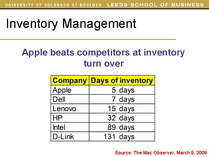
Inventory Management Apple beats competitors at inventory turn over Source: The Mac Observer, March 5, 2009

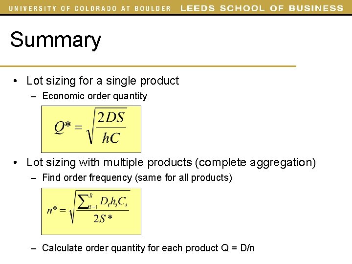
Summary • Lot sizing for a single product – Economic order quantity • Lot sizing with multiple products (complete aggregation) – Find order frequency (same for all products) – Calculate order quantity for each product Q = D/n

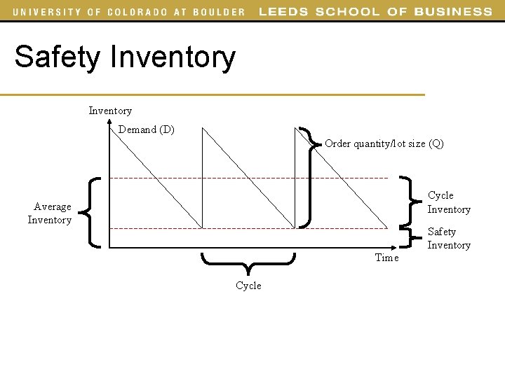
Safety Inventory Demand (D) Order quantity/lot size (Q) Cycle Inventory Average Inventory Safety Inventory Time Cycle

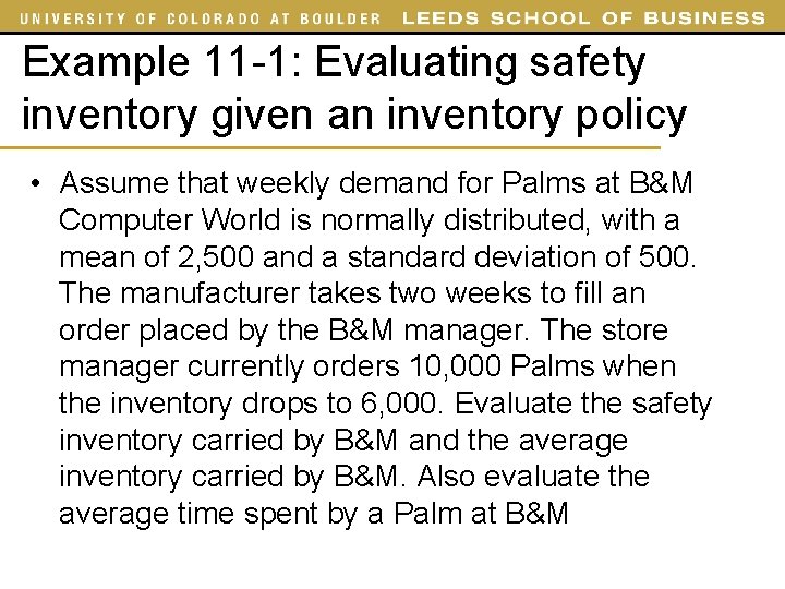
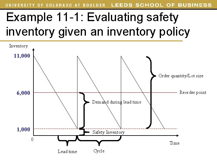
Example 11 -1: Evaluating safety inventory given an inventory policy • Assume that weekly demand for Palms at B&M Computer World is normally distributed, with a mean of 2, 500 and a standard deviation of 500. The manufacturer takes two weeks to fill an order placed by the B&M manager. The store manager currently orders 10, 000 Palms when the inventory drops to 6, 000. Evaluate the safety inventory carried by B&M and the average inventory carried by B&M. Also evaluate the average time spent by a Palm at B&M

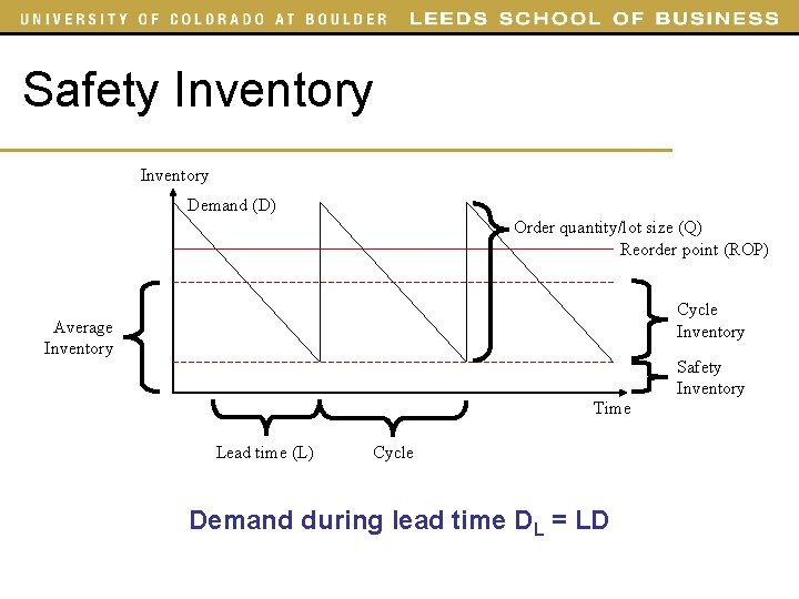
Safety Inventory Demand (D) Order quantity/lot size (Q) Reorder point (ROP) Cycle Inventory Average Inventory Safety Inventory Time Lead time (L) Cycle Demand during lead time DL = LD

Example 11 -1: Evaluating safety inventory given an inventory policy Inventory 11, 000 Order quantity/Lot size 6, 000 Reorder point Demand during lead time 1, 000 Safety Inventory 0 Time Lead time Cycle

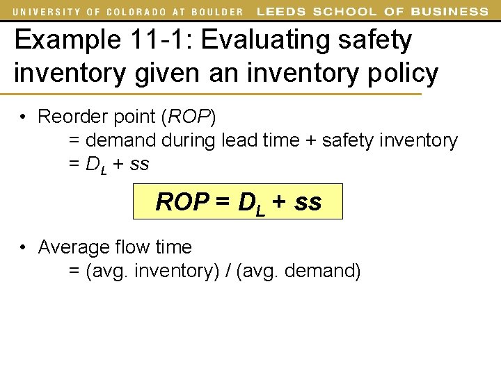
Example 11 -1: Evaluating safety inventory given an inventory policy • Reorder point (ROP) = demand during lead time + safety inventory = DL + ss ROP = DL + ss • Average flow time = (avg. inventory) / (avg. demand)

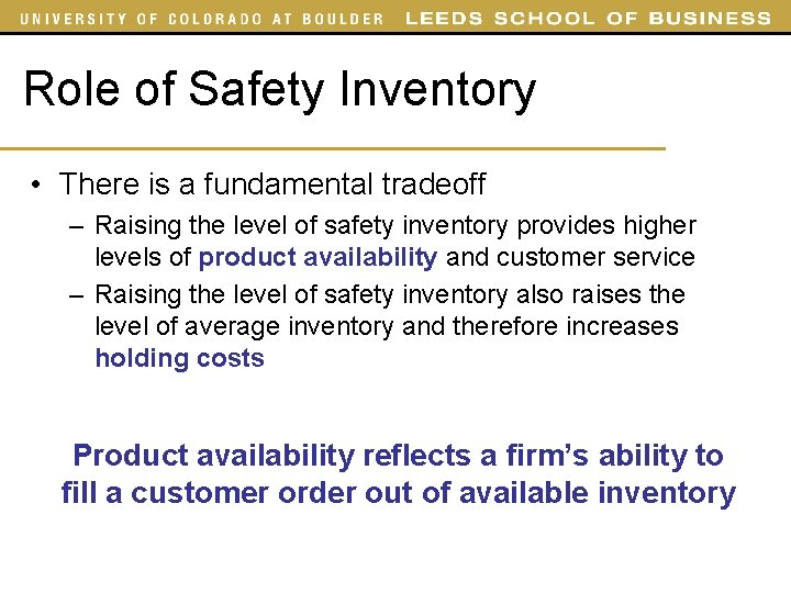
Role of Safety Inventory • There is a fundamental tradeoff – Raising the level of safety inventory provides higher levels of product availability and customer service – Raising the level of safety inventory also raises the level of average inventory and therefore increases holding costs Product availability reflects a firm’s ability to fill a customer order out of available inventory

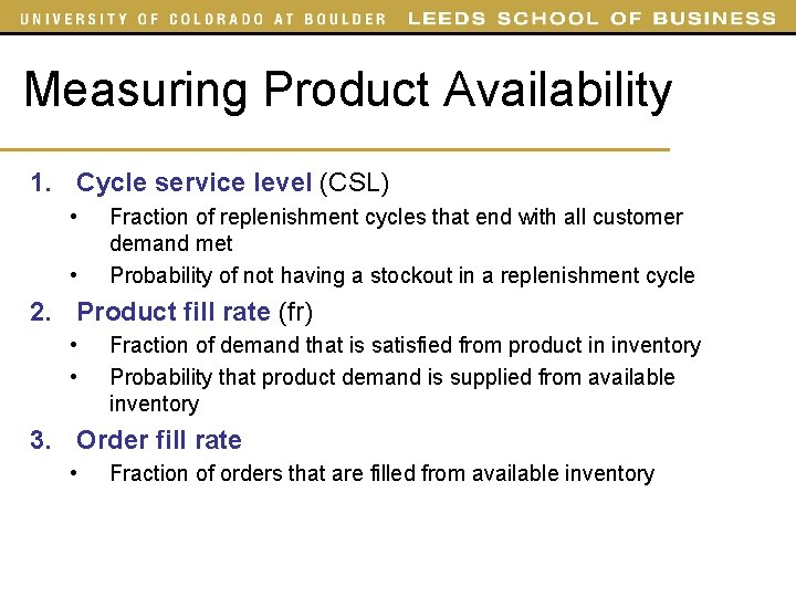
Measuring Product Availability 1. Cycle service level (CSL) • • Fraction of replenishment cycles that end with all customer demand met Probability of not having a stockout in a replenishment cycle 2. Product fill rate (fr) • • Fraction of demand that is satisfied from product in inventory Probability that product demand is supplied from available inventory 3. Order fill rate • Fraction of orders that are filled from available inventory

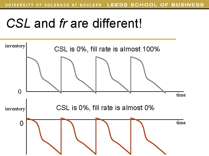
CSL and fr are different! inventory CSL is 0%, fill rate is almost 100% 0 inventory 0 time CSL is 0%, fill rate is almost 0% time

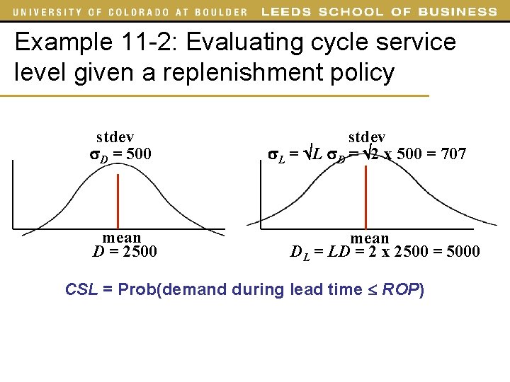
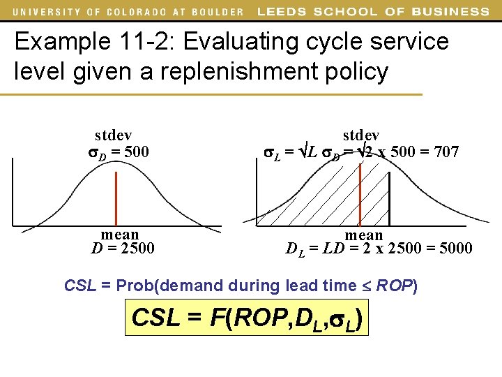
Example 11 -2: Evaluating cycle service level given a replenishment policy • Weekly demand for Palms is normally distributed, with a mean of 2, 500 and a standard deviation of 500. The replenishment lead time is two weeks. Assume that the demand is independent from one week to the next. Evaluate the CSL resulting from a policy of ordering 10, 000 Palms when there are 6, 000 Palms in inventory

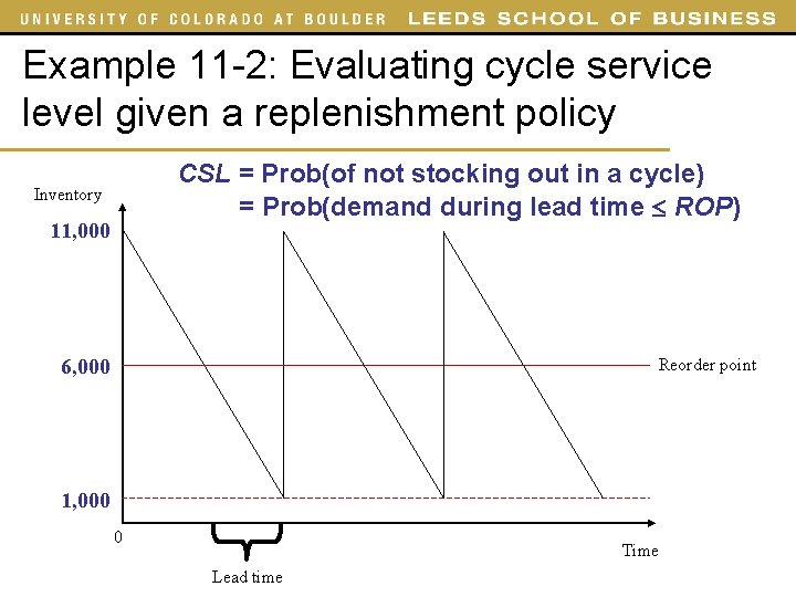
Example 11 -2: Evaluating cycle service level given a replenishment policy CSL = Prob(of not stocking out in a cycle) = Prob(demand during lead time ROP) Inventory 11, 000 6, 000 Reorder point 1, 000 0 Time Lead time

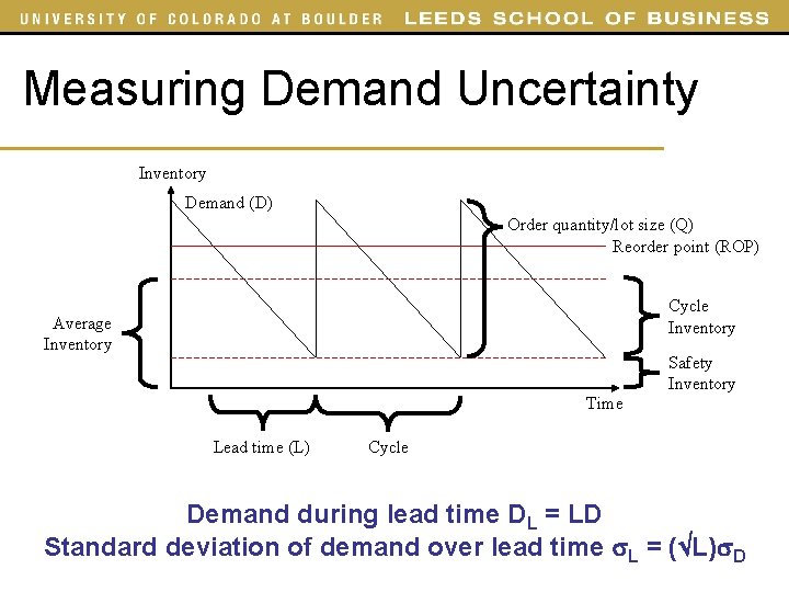
Measuring Demand Uncertainty Inventory Demand (D) Order quantity/lot size (Q) Reorder point (ROP) Cycle Inventory Average Inventory Safety Inventory Time Lead time (L) Cycle Demand during lead time DL = LD Standard deviation of demand over lead time L = ( L) D

Example 11 -2: Evaluating cycle service level given a replenishment policy stdev D = 500 mean D = 2500 stdev L = L D = 2 x 500 = 707 mean DL = LD = 2 x 2500 = 5000 CSL = Prob(demand during lead time ROP)

Example 11 -2: Evaluating cycle service level given a replenishment policy stdev D = 500 mean D = 2500 stdev L = L D = 2 x 500 = 707 mean DL = LD = 2 x 2500 = 5000 CSL = Prob(demand during lead time ROP) CSL = F(ROP, DL, L)

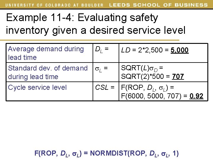
Example 11 -4: Evaluating safety inventory given a desired service level Average demand during lead time DL = LD = 2*2, 500 = 5, 000 Standard dev. of demand during lead time Cycle service level L = SQRT(L) D = SQRT(2)*500 = 707 CSL = F(ROP, DL, L) = F(6000, 5000, 707) = 0. 92 F(ROP, DL, L) = NORMDIST(ROP, DL, L, 1)

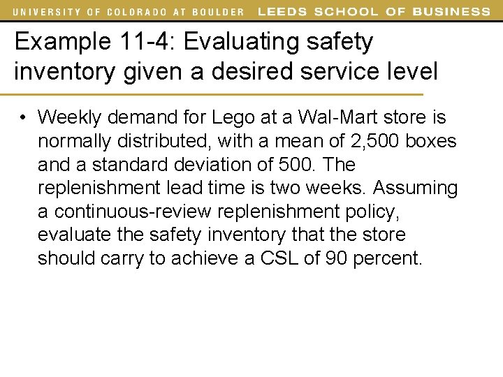
Example 11 -4: Evaluating safety inventory given a desired service level • Weekly demand for Lego at a Wal-Mart store is normally distributed, with a mean of 2, 500 boxes and a standard deviation of 500. The replenishment lead time is two weeks. Assuming a continuous-review replenishment policy, evaluate the safety inventory that the store should carry to achieve a CSL of 90 percent.

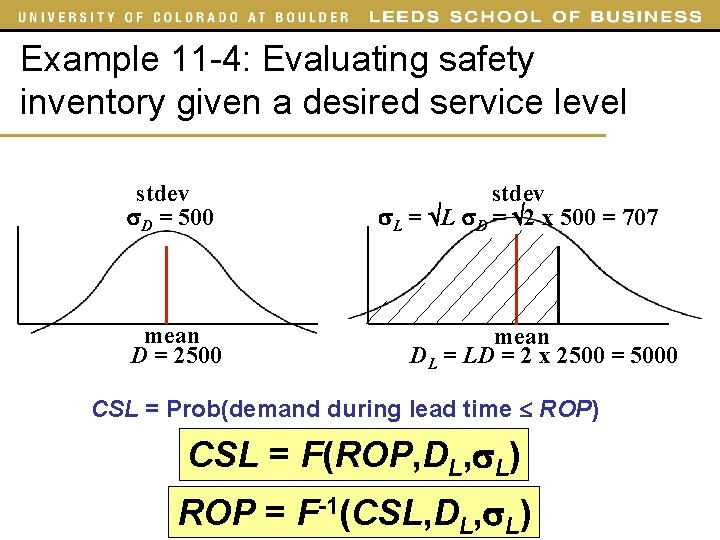
Example 11 -4: Evaluating safety inventory given a desired service level stdev D = 500 mean D = 2500 stdev L = L D = 2 x 500 = 707 mean DL = LD = 2 x 2500 = 5000 CSL = Prob(demand during lead time ROP) CSL = F(ROP, DL, L) ROP = F-1(CSL, DL, L)

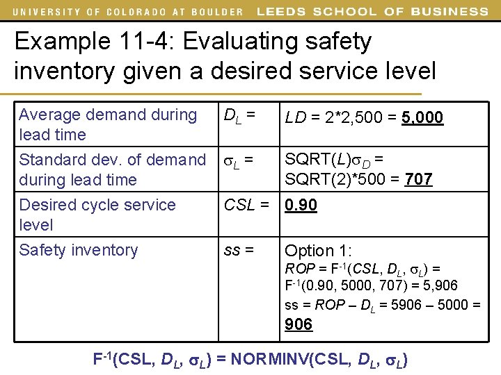
Example 11 -4: Evaluating safety inventory given a desired service level Average demand during lead time DL = LD = 2*2, 500 = 5, 000 Standard dev. of demand during lead time L = SQRT(L) D = SQRT(2)*500 = 707 Desired cycle service level Safety inventory CSL = 0. 90 ss = Option 1: ROP = F-1(CSL, DL, L) = F-1(0. 90, 5000, 707) = 5, 906 ss = ROP – DL = 5906 – 5000 = 906 F-1(CSL, DL, L) = NORMINV(CSL, DL, L)

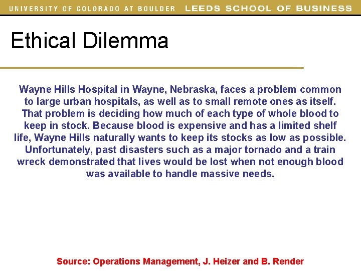
Ethical Dilemma Wayne Hills Hospital in Wayne, Nebraska, faces a problem common to large urban hospitals, as well as to small remote ones as itself. That problem is deciding how much of each type of whole blood to keep in stock. Because blood is expensive and has a limited shelf life, Wayne Hills naturally wants to keep its stocks as low as possible. Unfortunately, past disasters such as a major tornado and a train wreck demonstrated that lives would be lost when not enough blood was available to handle massive needs. Source: Operations Management, J. Heizer and B. Render

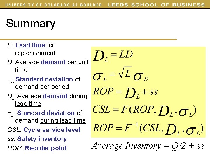
Summary L: Lead time for replenishment D: Average demand per unit time D: Standard deviation of demand period DL: Average demand during lead time L: Standard deviation of demand during lead time CSL: Cycle service level ss: Safety inventory ROP: Reorder point Average Inventory = Q/2 + ss

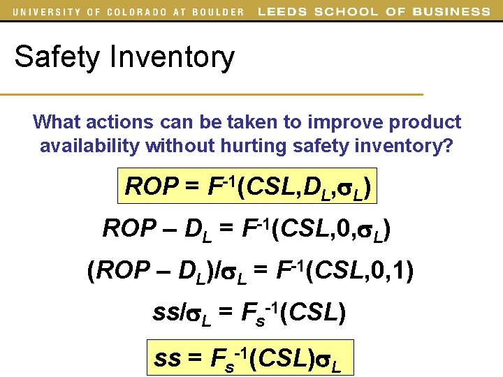
Safety Inventory What actions can be taken to improve product availability without hurting safety inventory? ROP = F-1(CSL, DL, L) ROP – DL = F-1(CSL, 0, L) (ROP – DL)/ L = F-1(CSL, 0, 1) ss/ L = Fs-1(CSL) ss = Fs-1(CSL) L

Safety Inventory Why is it that successful retailers and manufacturers (i. e. Wal-Mart, Seven-Eleven Japan, Dell) carry only little inventory but still have high levels of product availability?

Measuring Product Availability 1. Cycle service level (CSL) • • Fraction of replenishment cycles that end with all customer demand met Probability of not having a stockout in a replenishment cycle 2. Product fill rate (fr) • • Fraction of demand that is satisfied from product in inventory Probability that product demand is supplied from available inventory 3. Order fill rate • Fraction of orders that are filled from available inventory

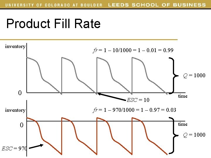
Product Fill Rate inventory fr = 1 – 10/1000 = 1 – 0. 01 = 0. 99 Q = 1000 0 ESC = 10 inventory 0 time fr = 1 – 970/1000 = 1 – 0. 97 = 0. 03 time Q = 1000 ESC = 970

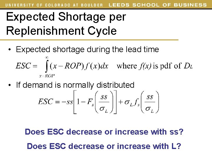
Expected Shortage per Replenishment Cycle • Expected shortage during the lead time • If demand is normally distributed Does ESC decrease or increase with ss? Does ESC decrease or increase with L?

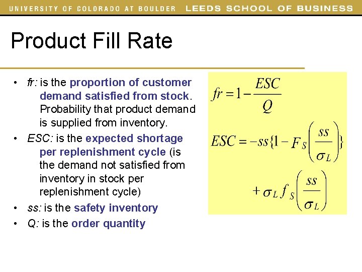
Product Fill Rate • fr: is the proportion of customer demand satisfied from stock. Probability that product demand is supplied from inventory. • ESC: is the expected shortage per replenishment cycle (is the demand not satisfied from inventory in stock per replenishment cycle) • ss: is the safety inventory • Q: is the order quantity

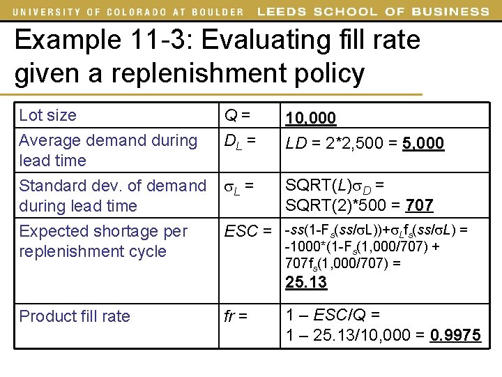
Example 11 -3: Evaluating fill rate given a replenishment policy • Recall that weekly demand for Palms at B&M is normally distributed, with a mean of 2, 500 and a standard deviation of 500. The replenishment lea time is two weeks. Assume that the demand is independent from one week to the next. Evaluate the fill rate resulting from the policy of ordering 10, 000 Palms when there are 6, 000 Palms in inventory.

Example 11 -3: Evaluating fill rate given a replenishment policy Lot size Average demand during lead time Q= DL = 10, 000 LD = 2*2, 500 = 5, 000 Standard dev. of demand during lead time Expected shortage per replenishment cycle L = SQRT(L) D = SQRT(2)*500 = 707 ESC = -ss(1 -Fs(ss/ L))+ Lfs(ss/ L) = -1000*(1 -Fs(1, 000/707) + 707 fs(1, 000/707) = 25. 13 Product fill rate fr = 1 – ESC/Q = 1 – 25. 13/10, 000 = 0. 9975

Cycle Service Level versus Fill Rate What happens to CSL and fr when the safety inventory (ss) increases? What happens to CSL and fr when the lot size (Q) increases?

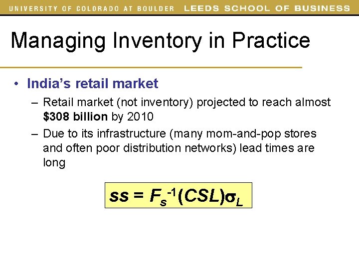
Managing Inventory in Practice • India’s retail market – Retail market (not inventory) projected to reach almost $308 billion by 2010 – Due to its infrastructure (many mom-and-pop stores and often poor distribution networks) lead times are long ss = Fs-1(CSL) L

Managing Inventory in Practice • Department of Defense – DOD reported (1995) that it had a secondary inventory (spare and repair parts, clothing, medical supplies, and other items) to support its operating forces valued at $69. 6 billion – About half of the inventory includes items that are not needed to be on hand to support DOD war reserve or current operating requirements