Supply Chain Management Chapter 8 Aggregate Planning in

Supply Chain Management Chapter 8 Aggregate Planning in the Supply Chain 8 -1

Production System u In a broader sense, a production system is anything that takes inputs and transforms them into outputs. u Production system is the collection of people, equipment, and procedures organized to accomplish the operations of a company (or other organization). – Manufacturing – Service 8 -2

Production Planning u Production Planning is the analysis, design and management of production systems. Objective: Transform a variety of inputs (such as raw material, labor, capital, etc. ) into outputs (goods and services) in a manner that is both efficient in using resources and effective in achieving high customer satisfaction. u In today’s competitive business environment it is important to know methods and specific analysis tools for operational decisions to effectively manage these systems. 8 -3

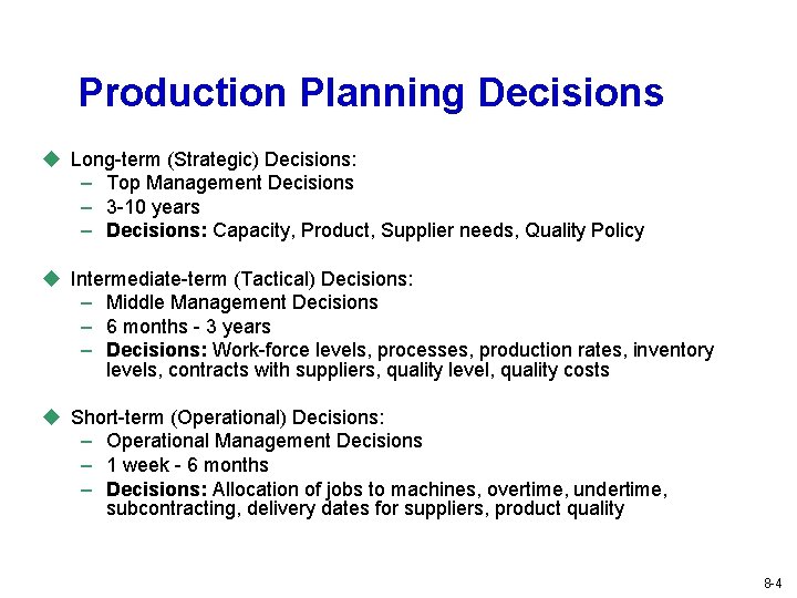
Production Planning Decisions u Long-term (Strategic) Decisions: – Top Management Decisions – 3 -10 years – Decisions: Capacity, Product, Supplier needs, Quality Policy u Intermediate-term (Tactical) Decisions: – Middle Management Decisions – 6 months - 3 years – Decisions: Work-force levels, processes, production rates, inventory levels, contracts with suppliers, quality level, quality costs u Short-term (Operational) Decisions: – Operational Management Decisions – 1 week - 6 months – Decisions: Allocation of jobs to machines, overtime, undertime, subcontracting, delivery dates for suppliers, product quality 8 -4

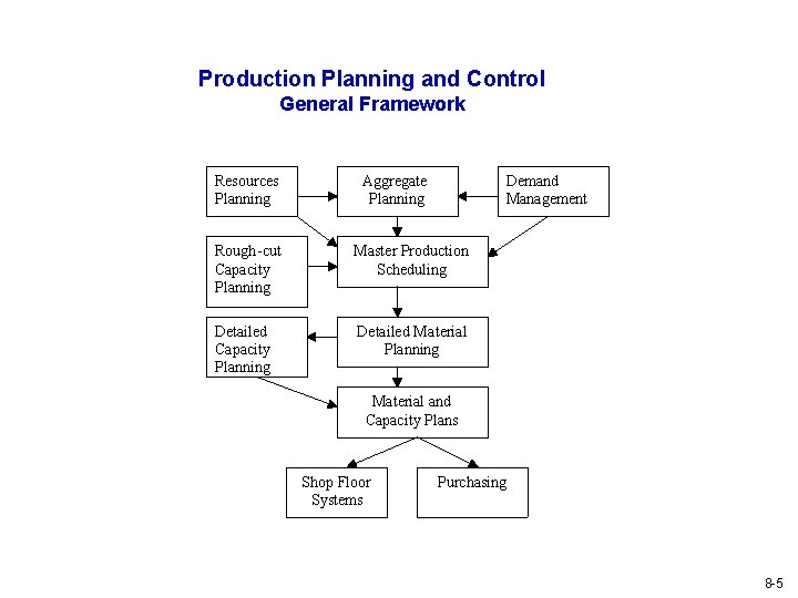
Production Planning and Control General Framework Resources Planning Rough-cut Capacity Planning Detailed Capacity Planning Aggregate Planning Demand Management Master Production Scheduling Detailed Material Planning Material and Capacity Plans Shop Floor Systems Purchasing 8 -5

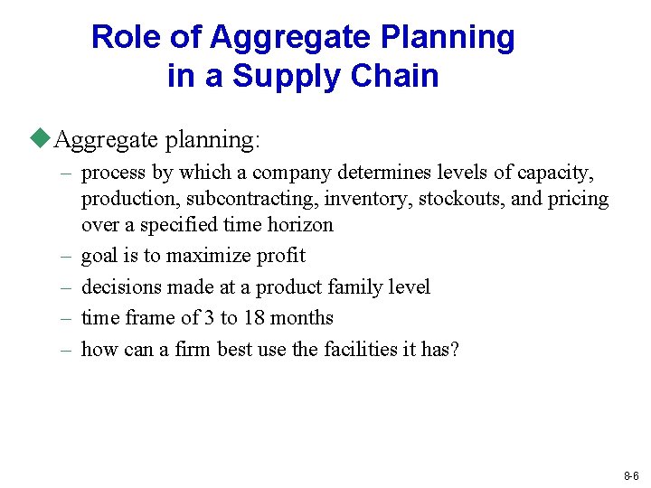
Role of Aggregate Planning in a Supply Chain u. Aggregate planning: – process by which a company determines levels of capacity, production, subcontracting, inventory, stockouts, and pricing over a specified time horizon – goal is to maximize profit – decisions made at a product family level – time frame of 3 to 18 months – how can a firm best use the facilities it has? 8 -6

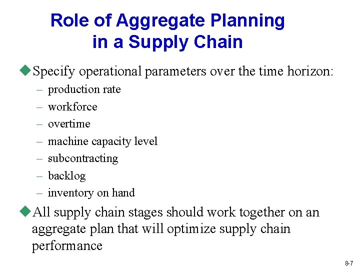
Role of Aggregate Planning in a Supply Chain u. Specify operational parameters over the time horizon: – – – – production rate workforce overtime machine capacity level subcontracting backlog inventory on hand u. All supply chain stages should work together on an aggregate plan that will optimize supply chain performance 8 -7

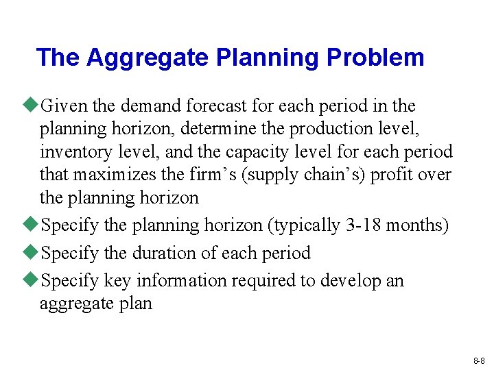
The Aggregate Planning Problem u. Given the demand forecast for each period in the planning horizon, determine the production level, inventory level, and the capacity level for each period that maximizes the firm’s (supply chain’s) profit over the planning horizon u. Specify the planning horizon (typically 3 -18 months) u. Specify the duration of each period u. Specify key information required to develop an aggregate plan 8 -8

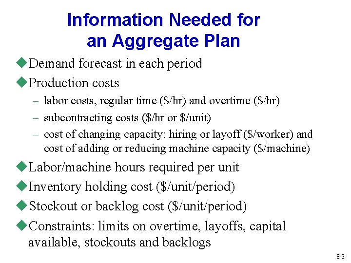
Information Needed for an Aggregate Plan u. Demand forecast in each period u. Production costs – labor costs, regular time ($/hr) and overtime ($/hr) – subcontracting costs ($/hr or $/unit) – cost of changing capacity: hiring or layoff ($/worker) and cost of adding or reducing machine capacity ($/machine) u. Labor/machine hours required per unit u. Inventory holding cost ($/unit/period) u. Stockout or backlog cost ($/unit/period) u. Constraints: limits on overtime, layoffs, capital available, stockouts and backlogs 8 -9

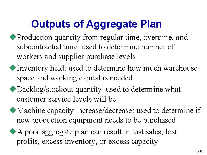
Outputs of Aggregate Plan u. Production quantity from regular time, overtime, and subcontracted time: used to determine number of workers and supplier purchase levels u. Inventory held: used to determine how much warehouse space and working capital is needed u. Backlog/stockout quantity: used to determine what customer service levels will be u. Machine capacity increase/decrease: used to determine if new production equipment needs to be purchased u. A poor aggregate plan can result in lost sales, lost profits, excess inventory, or excess capacity 8 -10

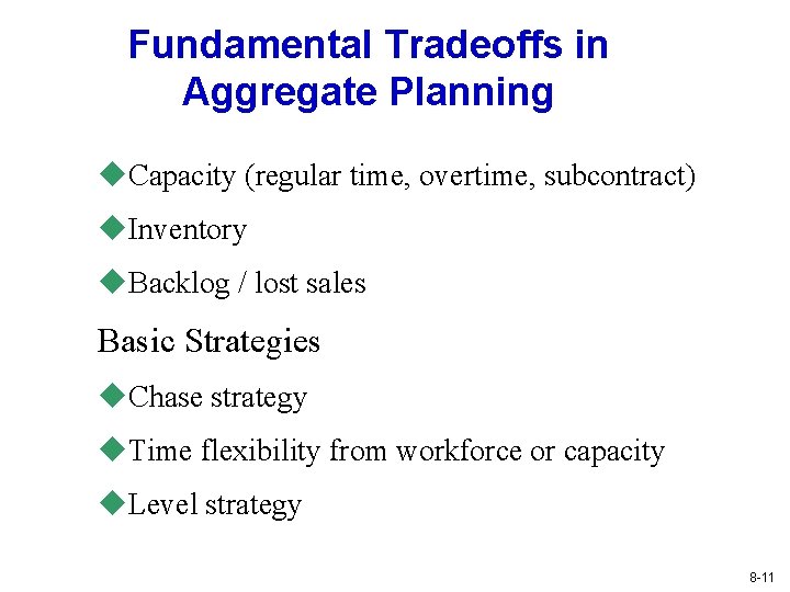
Fundamental Tradeoffs in Aggregate Planning u. Capacity (regular time, overtime, subcontract) u. Inventory u. Backlog / lost sales Basic Strategies u. Chase strategy u. Time flexibility from workforce or capacity u. Level strategy 8 -11

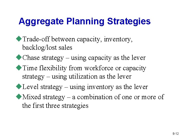
Aggregate Planning Strategies u. Trade-off between capacity, inventory, backlog/lost sales u. Chase strategy – using capacity as the lever u. Time flexibility from workforce or capacity strategy – using utilization as the lever u. Level strategy – using inventory as the lever u. Mixed strategy – a combination of one or more of the first three strategies 8 -12

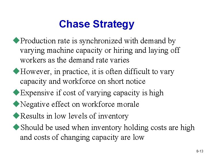
Chase Strategy u. Production rate is synchronized with demand by varying machine capacity or hiring and laying off workers as the demand rate varies u. However, in practice, it is often difficult to vary capacity and workforce on short notice u. Expensive if cost of varying capacity is high u. Negative effect on workforce morale u. Results in low levels of inventory u. Should be used when inventory holding costs are high and costs of changing capacity are low 8 -13

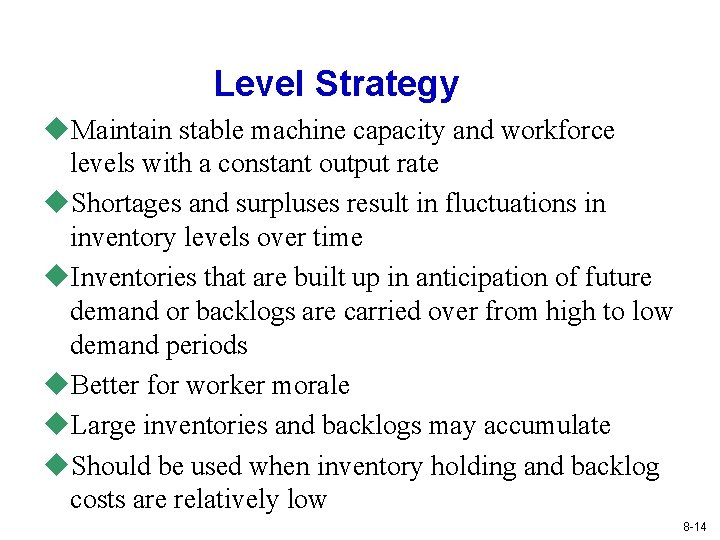
Level Strategy u. Maintain stable machine capacity and workforce levels with a constant output rate u. Shortages and surpluses result in fluctuations in inventory levels over time u. Inventories that are built up in anticipation of future demand or backlogs are carried over from high to low demand periods u. Better for worker morale u. Large inventories and backlogs may accumulate u. Should be used when inventory holding and backlog costs are relatively low 8 -14

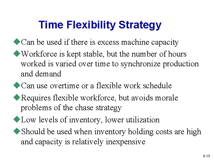
Time Flexibility Strategy u. Can be used if there is excess machine capacity u. Workforce is kept stable, but the number of hours worked is varied over time to synchronize production and demand u. Can use overtime or a flexible work schedule u. Requires flexible workforce, but avoids morale problems of the chase strategy u. Low levels of inventory, lower utilization u. Should be used when inventory holding costs are high and capacity is relatively inexpensive 8 -15

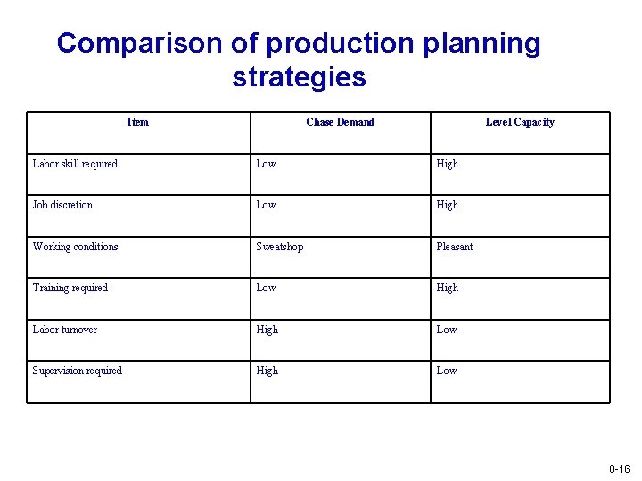
Comparison of production planning strategies Item Chase Demand Level Capacity Labor skill required Low High Job discretion Low High Working conditions Sweatshop Pleasant Training required Low High Labor turnover High Low Supervision required High Low 8 -16

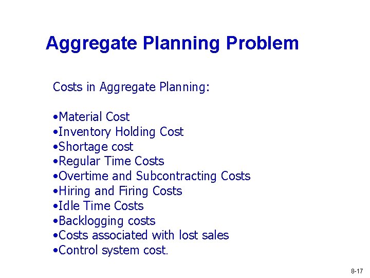
Aggregate Planning Problem Costs in Aggregate Planning: • Material Cost • Inventory Holding Cost • Shortage cost • Regular Time Costs • Overtime and Subcontracting Costs • Hiring and Firing Costs • Idle Time Costs • Backlogging costs • Costs associated with lost sales • Control system cost. 8 -17

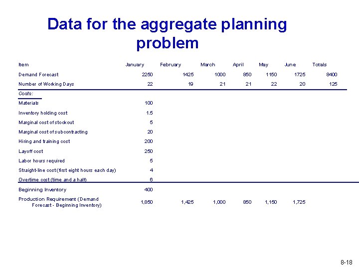
Data for the aggregate planning problem Item Demand Forecast Number of Working Days January February March April May June Totals 2250 1425 1000 850 1150 1725 8400 22 19 21 21 22 20 125 1, 425 1, 000 850 1, 150 1, 725 Costs: Materials 100 Inventory holding cost 1. 5 Marginal cost of stockout Marginal cost of subcontracting 5 20 Hiring and training cost 200 Layoff cost 250 Labor hours required 5 Straight-line cost (first eight hours each day) 4 Overtime cost (time and a half) 6 Beginning Inventory Production Requirement (Demand Forecast - Beginning Inventory) 400 1, 850 8 -18

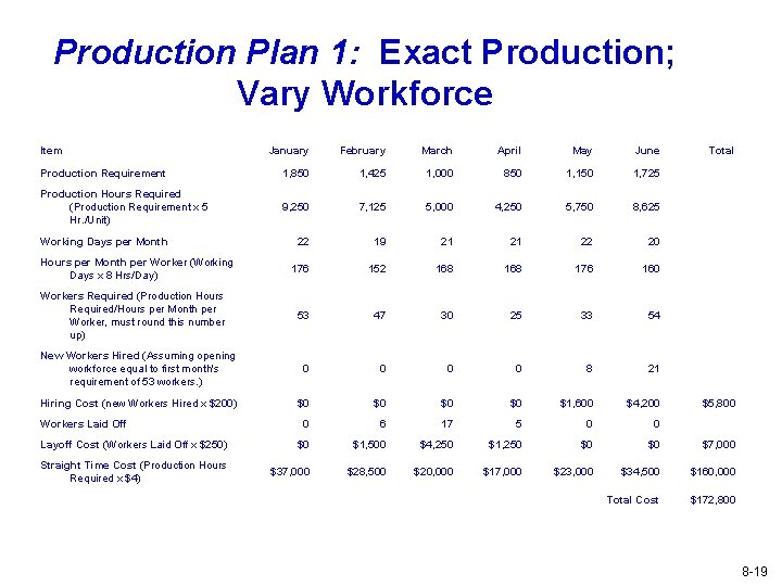
Production Plan 1: Exact Production; Vary Workforce Item January February March April May June Production Requirement 1, 850 1, 425 1, 000 850 1, 150 1, 725 Production Hours Required (Production Requirement x 5 Hr. /Unit) 9, 250 7, 125 5, 000 4, 250 5, 750 8, 625 22 19 21 21 22 20 176 152 168 176 160 53 47 30 25 33 54 New Workers Hired (Assuming opening workforce equal to first month's requirement of 53 workers. ) 0 0 8 21 Hiring Cost (new Workers Hired x $200) $0 $0 $1, 600 $4, 200 0 6 17 5 0 0 Layoff Cost (Workers Laid Off x $250) $0 $1, 500 $4, 250 $1, 250 $0 $0 $7, 000 Straight Time Cost (Production Hours Required x $4) $37, 000 $28, 500 $20, 000 $17, 000 $23, 000 $34, 500 $160, 000 Total Cost $172, 800 Working Days per Month Hours per Month per Worker (Working Days x 8 Hrs/Day) Workers Required (Production Hours Required/Hours per Month per Worker, must round this number up) Workers Laid Off Total $5, 800 8 -19

8 -20

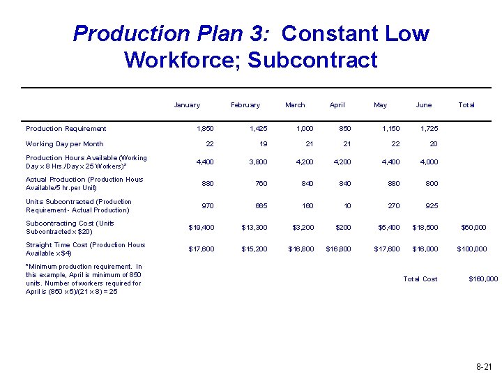
Production Plan 3: Constant Low Workforce; Subcontract Production Requirement January February March April May June Total 1, 850 1, 425 1, 000 850 1, 150 1, 725 22 19 21 21 22 20 4, 400 3, 800 4, 200 4, 400 4, 000 Actual Production (Production Hours Available/5 hr. per Unit) 880 760 840 880 800 Units Subcontracted (Production Requirement - Actual Production) 970 665 160 10 270 925 Subcontracting Cost (Units Subcontracted x $20) $19, 400 $13, 300 $3, 200 $5, 400 $18, 500 $60, 000 Straight Time Cost (Production Hours Available x $4) $17, 600 $15, 200 $16, 800 $17, 600 $16, 000 $100, 000 Working Day per Month Production Hours Available (Working Day x 8 Hrs. /Day x 25 Workers)* *Minimum production requirement. In this example, April is minimum of 850 units. Number of workers required for April is (850 x 5)/(21 x 8) = 25 Total Cost $160, 000 8 -21

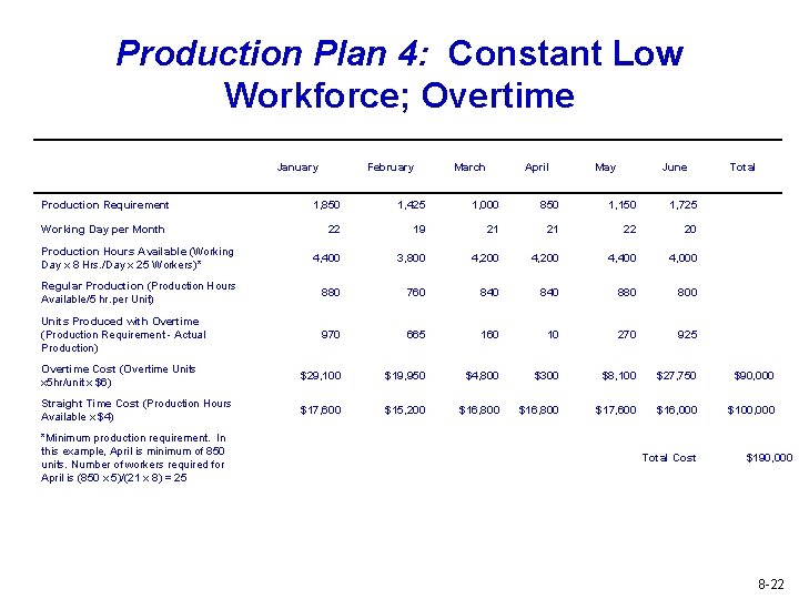
Production Plan 4: Constant Low Workforce; Overtime Production Requirement January February March April May June Total 1, 850 1, 425 1, 000 850 1, 150 1, 725 22 19 21 21 22 20 Production Hours Available (Working Day x 8 Hrs. /Day x 25 Workers)* 4, 400 3, 800 4, 200 4, 400 4, 000 Regular Production (Production Hours Available/5 hr. per Unit) 880 760 840 880 800 Units Produced with Overtime (Production Requirement - Actual Production) 970 665 160 10 270 925 Overtime Cost (Overtime Units x 5 hr/unit x $6) $29, 100 $19, 950 $4, 800 $300 $8, 100 $27, 750 $90, 000 Straight Time Cost (Production Hours Available x $4) $17, 600 $15, 200 $16, 800 $17, 600 $16, 000 $100, 000 Working Day per Month *Minimum production requirement. In this example, April is minimum of 850 units. Number of workers required for April is (850 x 5)/(21 x 8) = 25 Total Cost $190, 000 8 -22

Aggregate Planning at Red Tomato Tools 8 -23

Aggregate Planning 8 -24

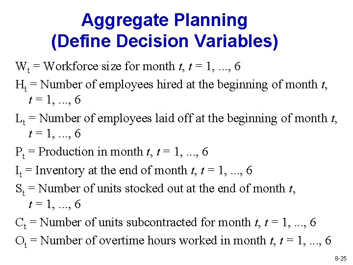
Aggregate Planning (Define Decision Variables) Wt = Workforce size for month t, t = 1, . . . , 6 Ht = Number of employees hired at the beginning of month t, t = 1, . . . , 6 Lt = Number of employees laid off at the beginning of month t, t = 1, . . . , 6 Pt = Production in month t, t = 1, . . . , 6 It = Inventory at the end of month t, t = 1, . . . , 6 St = Number of units stocked out at the end of month t, t = 1, . . . , 6 Ct = Number of units subcontracted for month t, t = 1, . . . , 6 Ot = Number of overtime hours worked in month t, t = 1, . . . , 6 8 -25

Aggregate Planning (Define Objective Function) 8 -26

Aggregate Planning (Define Constraints Linking Variables) u. Workforce size for each month is based on hiring and layoffs 8 -27

Aggregate Planning (Constraints) u. Production for each month cannot exceed capacity 8 -28

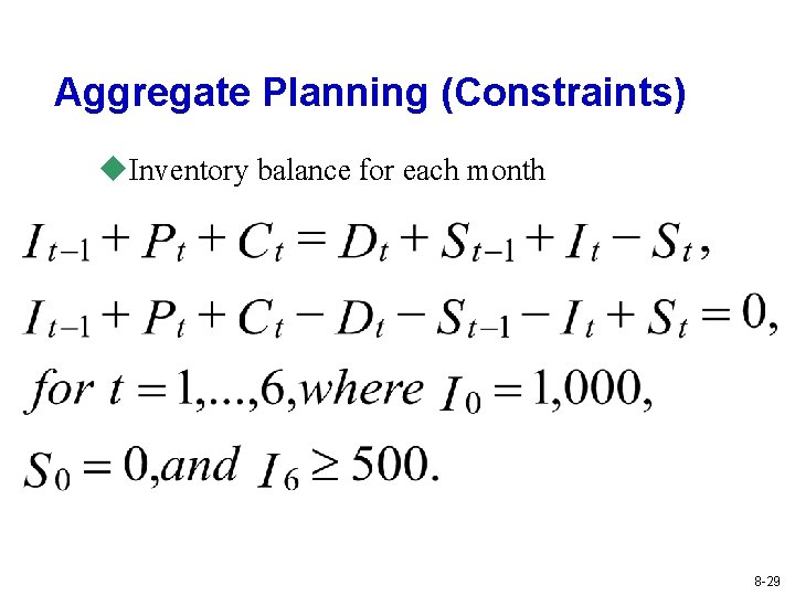
Aggregate Planning (Constraints) u. Inventory balance for each month 8 -29

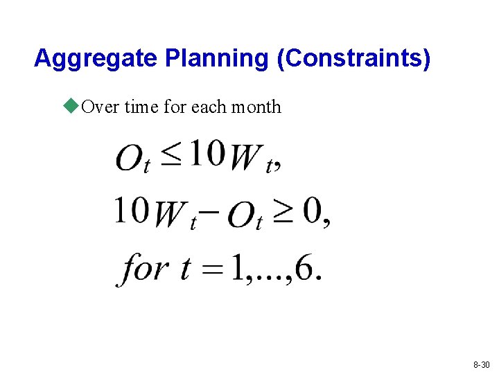
Aggregate Planning (Constraints) u. Over time for each month 8 -30

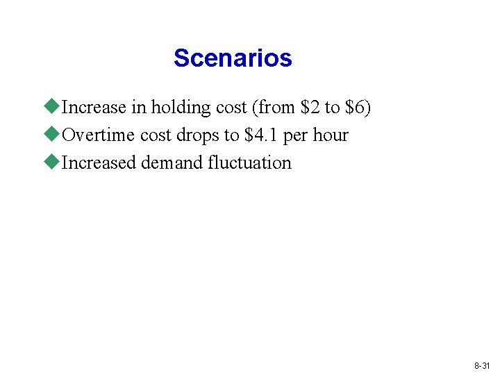
Scenarios u. Increase in holding cost (from $2 to $6) u. Overtime cost drops to $4. 1 per hour u. Increased demand fluctuation 8 -31

Increased Demand Fluctuation 8 -32

Aggregate Planning in Practice u. Think beyond the enterprise to the entire supply chain u. Make plans flexible because forecasts are always wrong u. Rerun the aggregate plan as new information emerges u. Use aggregate planning as capacity utilization increases 8 -33

Production Planning and Control General Framework Resources Planning Rough-cut Capacity Planning Detailed Capacity Planning Aggregate Planning Demand Management Master Production Scheduling Detailed Material Planning Material and Capacity Plans Shop Floor Systems Purchasing 8 -34

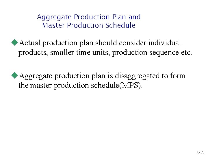
Aggregate Production Plan and Master Production Schedule u. Actual production plan should consider individual products, smaller time units, production sequence etc. u. Aggregate production plan is disaggregated to form the master production schedule(MPS). 8 -35

Aggregate Production Plan and Master Production Schedule 8 -36

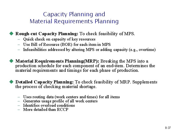
Capacity Planning and Material Requirements Planning u Rough-cut Capacity Planning: To check feasibility of MPS. – Quick check on capacity of key resources – Use Bill of Resource (BOR) for each item in MPS – Infeasibilities addressed by altering MPS or adding capacity (e. g. , overtime) u Material Requirements Planning(MRP): Breaking the MPS into a production schedule for each component of an end-item. Determines the material requirements and timings for each phase of production. u Detailed Capacity Planning: To check feasibility of MRP. Supplements the process of checking material shortage. – – Uses routing data (work centers and times) for all items Generates usage profile of all work centers Identifies overload conditions More detailed than RCCP 8 -37

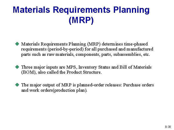
Materials Requirements Planning (MRP) u Materials Requirements Planning (MRP) determines time-phased requirements (period-by-period) for all purchased and manufactured parts such as raw materials, components, parts, subassemblies, etc. u Three major inputs are MPS, Inventory Status and Bill of Materials (BOM), also called the Product Structure. u The major output of MRP is planned-order releases: Purchase orders and work orders(production plan). 8 -38

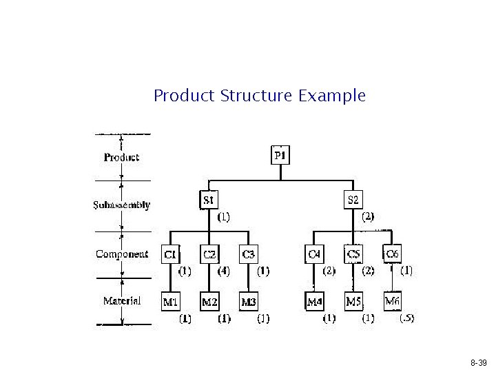
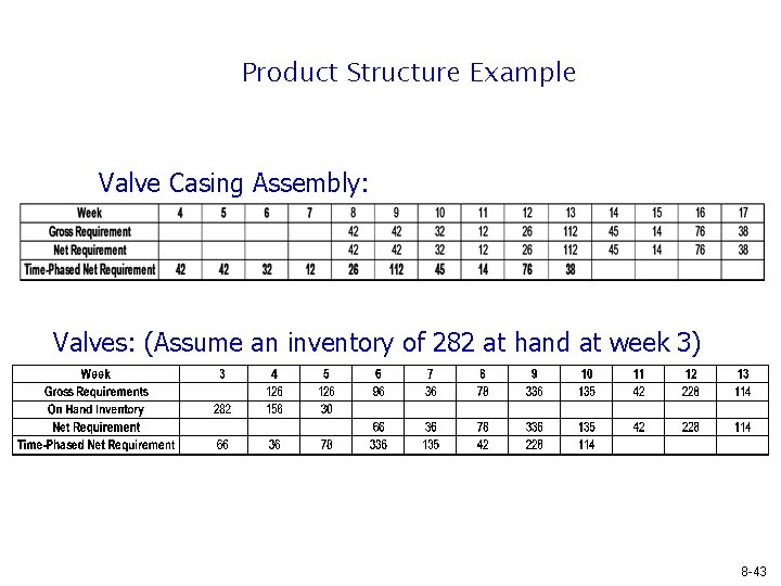
Product Structure Example 8 -39

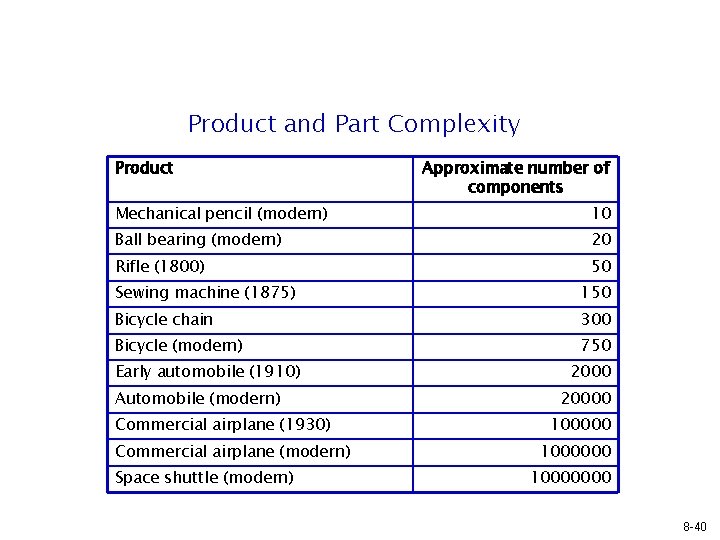
Product and Part Complexity Product Approximate number of components Mechanical pencil (modern) 10 Ball bearing (modern) 20 Rifle (1800) 50 Sewing machine (1875) 150 Bicycle chain 300 Bicycle (modern) 750 Early automobile (1910) Automobile (modern) Commercial airplane (1930) Commercial airplane (modern) Space shuttle (modern) 20000 10000000 8 -40

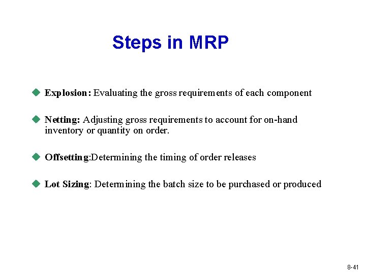
Steps in MRP u Explosion: Evaluating the gross requirements of each component u Netting: Adjusting gross requirements to account for on-hand inventory or quantity on order. u Offsetting: Determining the timing of order releases u Lot Sizing: Determining the batch size to be purchased or produced 8 -41

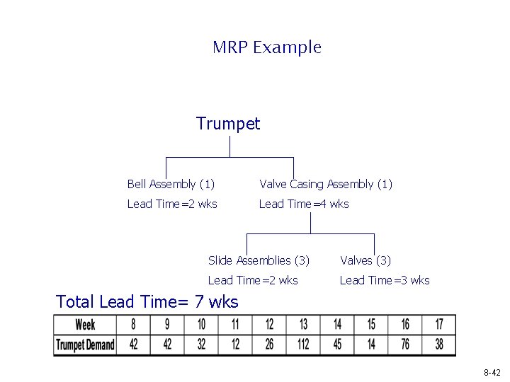
MRP Example Trumpet Bell Assembly (1) Valve Casing Assembly (1) Lead Time=2 wks Lead Time=4 wks Slide Assemblies (3) Valves (3) Lead Time=2 wks Lead Time=3 wks Total Lead Time= 7 wks 8 -42

Product Structure Example Valve Casing Assembly: Valves: (Assume an inventory of 282 at hand at week 3) 8 -43

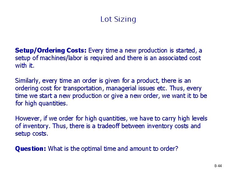
Lot Sizing Setup/Ordering Costs: Every time a new production is started, a setup of machines/labor is required and there is an associated cost with it. Similarly, every time an order is given for a product, there is an ordering cost for transportation, managerial issues etc. Thus, every time we start a new production or give a new order, we want it to be for high quantities. However, if we order for high quantities, we have to carry high levels of inventory. Thus, there is a tradeoff between inventory costs and setup costs. Question: What is the optimal time and amount to order? 8 -44

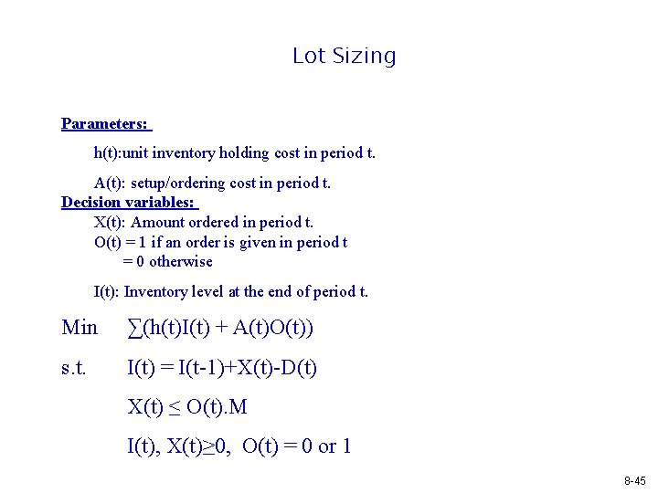
Lot Sizing Parameters: h(t): unit inventory holding cost in period t. A(t): setup/ordering cost in period t. Decision variables: X(t): Amount ordered in period t. O(t) = 1 if an order is given in period t = 0 otherwise I(t): Inventory level at the end of period t. Min ∑(h(t)I(t) + A(t)O(t)) s. t. I(t) = I(t-1)+X(t)-D(t) X(t) ≤ O(t). M I(t), X(t)≥ 0, O(t) = 0 or 1 8 -45

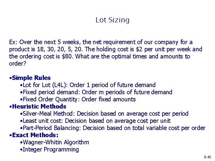
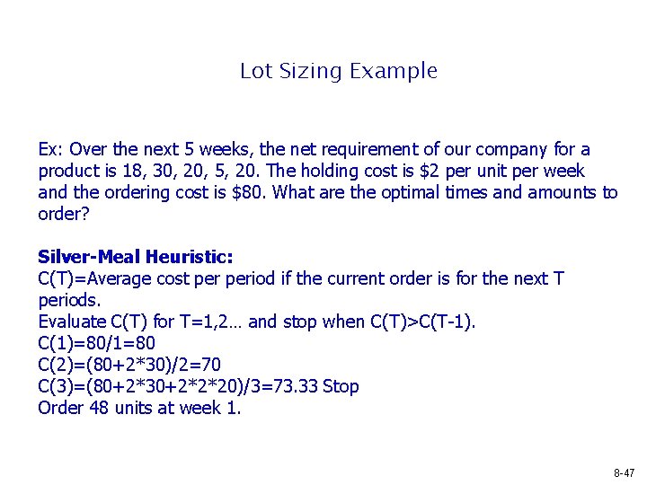
Lot Sizing Ex: Over the next 5 weeks, the net requirement of our company for a product is 18, 30, 20, 5, 20. The holding cost is $2 per unit per week and the ordering cost is $80. What are the optimal times and amounts to order? • Simple Rules • Lot for Lot (L 4 L): Order 1 period of future demand • Fixed period demand: Order m periods of future demand • Fixed Order Quantity: Order fixed amounts • Heuristic Methods • Silver-Meal Method: Decision based on average cost period • Least unit cost: Decision based on average cost per unit • Part-Period Balancing: Decision based on total variable cost per order • Exact Methods: • Wagner-Whitin Algorithm • Integer Programming 8 -46

Lot Sizing Example Ex: Over the next 5 weeks, the net requirement of our company for a product is 18, 30, 20, 5, 20. The holding cost is $2 per unit per week and the ordering cost is $80. What are the optimal times and amounts to order? Silver-Meal Heuristic: C(T)=Average cost period if the current order is for the next T periods. Evaluate C(T) for T=1, 2… and stop when C(T)>C(T-1). C(1)=80/1=80 C(2)=(80+2*30)/2=70 C(3)=(80+2*30+2*2*20)/3=73. 33 Stop Order 48 units at week 1. 8 -47

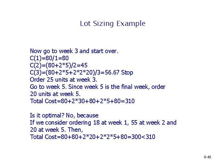
Lot Sizing Example Now go to week 3 and start over. C(1)=80/1=80 C(2)=(80+2*5)/2=45 C(3)=(80+2*5+2*2*20)/3=56. 67 Stop Order 25 units at week 3. Go to week 5. Since week 5 is the final week, order 20 units at week 5. Total Cost=80+2*30+80+2*5+80=310 Is it optimal? No, because If we consider ordering 18 at week 1, 55 at week 2 and 20 at week 5. Then, Total Cost=80+80+2*2*5+80=300<310 8 -48

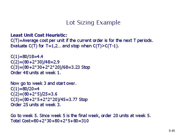
Lot Sizing Example Least Unit Cost Heuristic: C(T)=Average cost per unit if the current order is for the next T periods. Evaluate C(T) for T=1, 2… and stop when C(T)>C(T-1). C(1)=80/18=4. 4 C(2)=(80+2*30)/48=2. 9 C(3)=(80+2*30+2*2*20)/68=3. 23 Stop Order 48 units at week 1. Now go to week 3 and start over. C(1)=80/20=4 C(2)=(80+2*5)/25=3. 6 C(3)=(80+2*5+2*2*20)/45=3. 77 Stop Order 25 units at week 3. Go to week 5. Since week 5 is the final week, order 20 units at week 5. Total Cost=80+2*30+80+2*5+80=310 8 -49

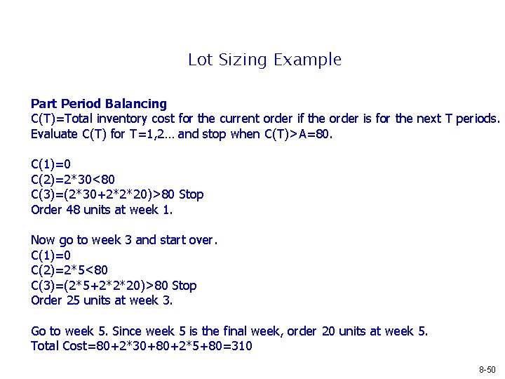
Lot Sizing Example Part Period Balancing C(T)=Total inventory cost for the current order if the order is for the next T periods. Evaluate C(T) for T=1, 2… and stop when C(T)>A=80. C(1)=0 C(2)=2*30<80 C(3)=(2*30+2*2*20)>80 Stop Order 48 units at week 1. Now go to week 3 and start over. C(1)=0 C(2)=2*5<80 C(3)=(2*5+2*2*20)>80 Stop Order 25 units at week 3. Go to week 5. Since week 5 is the final week, order 20 units at week 5. Total Cost=80+2*30+80+2*5+80=310 8 -50

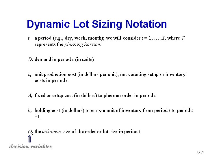
Dynamic Lot Sizing Notation t a period (e. g. , day, week, month); we will consider t = 1, … , T, where T represents the planning horizon. Dt demand in period t (in units) ct unit production cost (in dollars per unit), not counting setup or inventory costs in period t At fixed or setup cost (in dollars) to place an order in period t ht holding cost (in dollars) to carry a unit of inventory from period t to period t +1 Qt the unknown size of the order or lot size in period t decision variables 8 -51

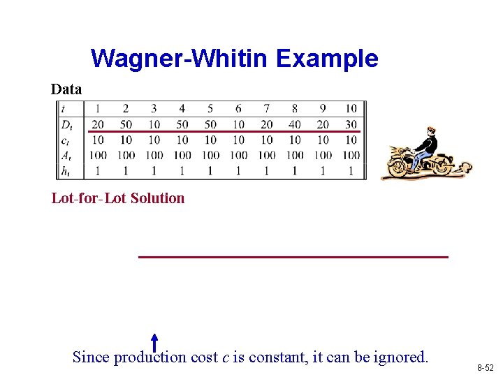
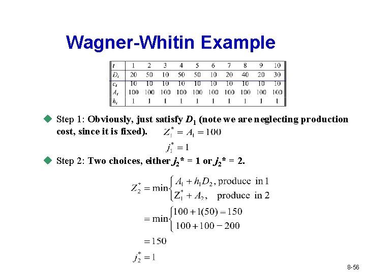
Wagner-Whitin Example Data Lot-for-Lot Solution Since production cost c is constant, it can be ignored. 8 -52

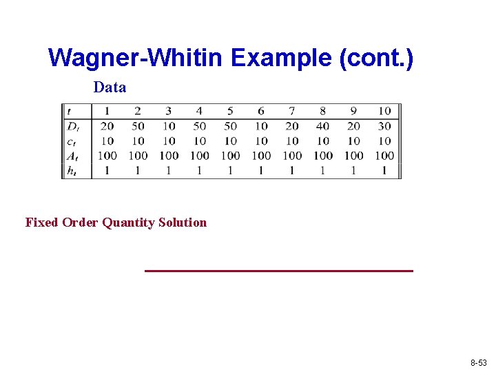
Wagner-Whitin Example (cont. ) Data Fixed Order Quantity Solution 8 -53

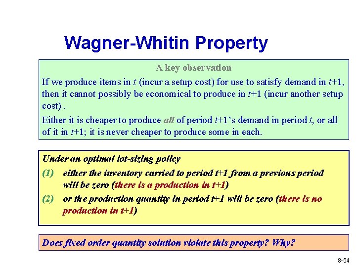
Wagner-Whitin Property A key observation If we produce items in t (incur a setup cost) for use to satisfy demand in t+1, then it cannot possibly be economical to produce in t+1 (incur another setup cost). Either it is cheaper to produce all of period t+1’s demand in period t, or all of it in t+1; it is never cheaper to produce some in each. Under an optimal lot-sizing policy (1) either the inventory carried to period t+1 from a previous period will be zero (there is a production in t+1) (2) or the production quantity in period t+1 will be zero (there is no production in t+1) Does fixed order quantity solution violate this property? Why? 8 -54

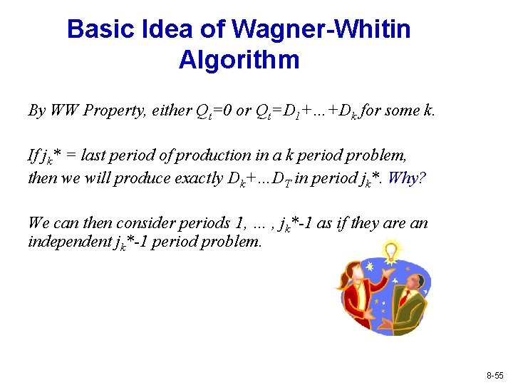
Basic Idea of Wagner-Whitin Algorithm By WW Property, either Qt=0 or Qt=D 1+…+Dk for some k. If jk* = last period of production in a k period problem, then we will produce exactly Dk+…DT in period jk*. Why? We can then consider periods 1, … , jk*-1 as if they are an independent jk*-1 period problem. 8 -55

Wagner-Whitin Example u Step 1: Obviously, just satisfy D 1 (note we are neglecting production cost, since it is fixed). u Step 2: Two choices, either j 2* = 1 or j 2* = 2. 8 -56

Wagner-Whitin Example (cont. ) u Step 3: Three choices, j 3* = 1, 2, 3. 8 -57

Wagner-Whitin Example (cont. ) u Step 4: Four choices, j 4* = 1, 2, 3, 4. 8 -58

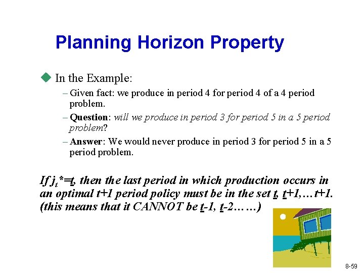
Planning Horizon Property u In the Example: – Given fact: we produce in period 4 for period 4 of a 4 period problem. – Question: will we produce in period 3 for period 5 in a 5 period problem? – Answer: We would never produce in period 3 for period 5 in a 5 period problem. If jt*=t, then the last period in which production occurs in an optimal t+1 period policy must be in the set t, t+1, …t+1. (this means that it CANNOT be t-1, t-2……) 8 -59

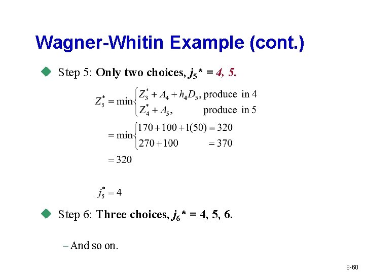
Wagner-Whitin Example (cont. ) u Step 5: Only two choices, j 5* = 4, 5. u Step 6: Three choices, j 6* = 4, 5, 6. – And so on. 8 -60

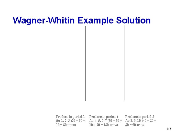
Wagner-Whitin Example Solution Produce in period 1 for 1, 2, 3 (20 + 50 + 10 = 80 units) Produce in period 4 Produce in period 8 for 4, 5, 6, 7 (50 + for 8, 9, 10 (40 + 20 + 10 + 20 = 130 units) 30 = 90 units 8 -61

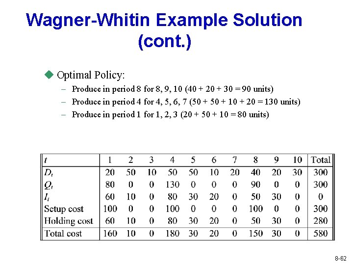
Wagner-Whitin Example Solution (cont. ) u Optimal Policy: – Produce in period 8 for 8, 9, 10 (40 + 20 + 30 = 90 units) – Produce in period 4 for 4, 5, 6, 7 (50 + 10 + 20 = 130 units) – Produce in period 1 for 1, 2, 3 (20 + 50 + 10 = 80 units) 8 -62