Supply Chain Logistics Systems GLBL 3250 Week 3

Supply Chain & Logistics Systems GLBL 3250 Week 3 Balancing Supply & Demand - Inventory

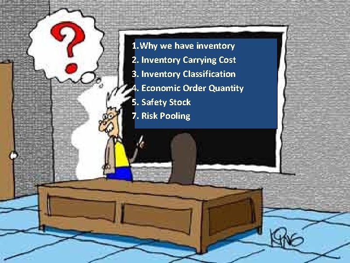
1. Why we have inventory 2. Inventory Carrying Cost 3. Inventory Classification 4. Economic Order Quantity 5. Safety Stock 7. Risk Pooling 2

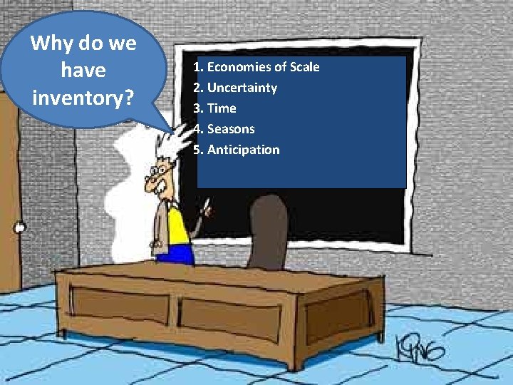
Why do we have inventory? 1. Economies of Scale 2. Uncertainty 3. Time 4. Seasons 5. Anticipation 3

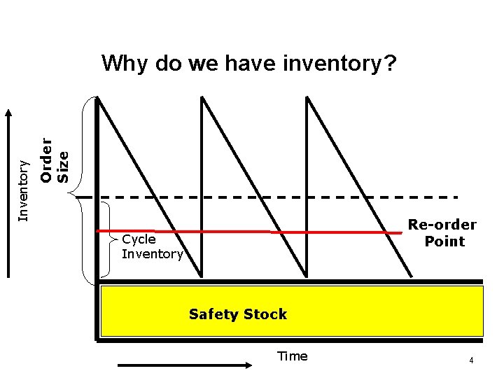
Order Size Inventory Why do we have inventory? Re-order Point Cycle Inventory Safety Stock Time 4

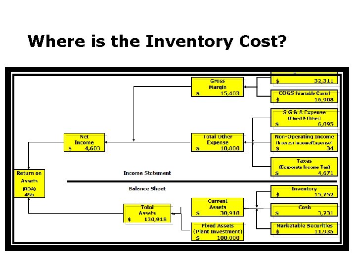
Where is the Inventory Cost?

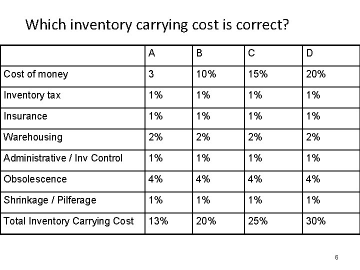
Which inventory carrying cost is correct? A B C D Cost of money 3 10% 15% 20% Inventory tax 1% 1% Insurance 1% 1% Warehousing 2% 2% Administrative / Inv Control 1% 1% Obsolescence 4% 4% Shrinkage / Pilferage 1% 1% Total Inventory Carrying Cost 13% 20% 25% 30% 6

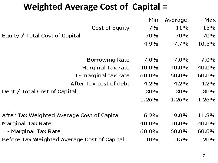
Weighted Average Cost of Capital = Min Cost of Equity Average Max 7% 11% 15% 70% 70% 4. 9% 7. 7% 10. 5% Borrowing Rate 7. 0% Marginal Tax rate 40. 0% 1 - marginal tax rate 60. 0% After Tax cost of debt 4. 2% 30% 30% 1. 26% 6. 2% 9. 0% 11. 8% Marginal Tax Rate 40. 0% 1 - Marginal Tax Rate 60. 0% 15% 20% Equity / Total Cost of Capital Debt / Total Cost of Capital After Tax Weighted Average Cost of Capital Before Tax Weighted Average Cost of Capital 7

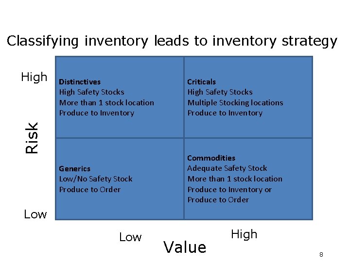
Classifying inventory leads to inventory strategy Distinctives High Safety Stocks More than 1 stock location Produce to Inventory Criticals High Safety Stocks Multiple Stocking locations Produce to Inventory Generics Low/No Safety Stock Produce to Order Commodities Adequate Safety Stock More than 1 stock location Produce to Inventory or Produce to Order Risk High Low Value High 8

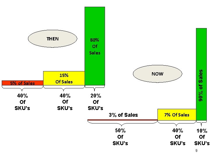
5% of Sales 15% Of Sales 40% Of SKU’s 80% Of Sales 90% of Sales THEN NOW 20% Of SKU’s 3% of Sales 50% Of SKU’s 7% Of Sales 40% Of SKU’s 10% Of SKU’s 9

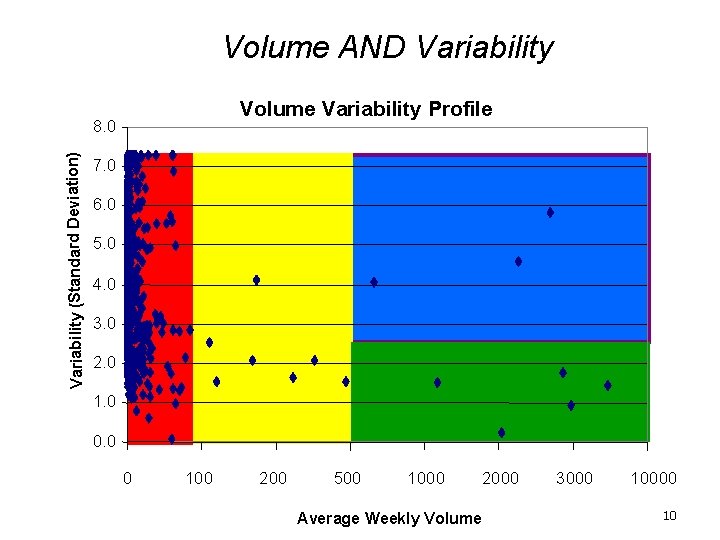
Volume AND Variability Volume Variability Profile Variability (Standard Deviation) 8. 0 7. 0 6. 0 5. 0 4. 0 3. 0 2. 0 1. 0 0 100 200 500 1000 2000 Average Weekly Volume 3000 10

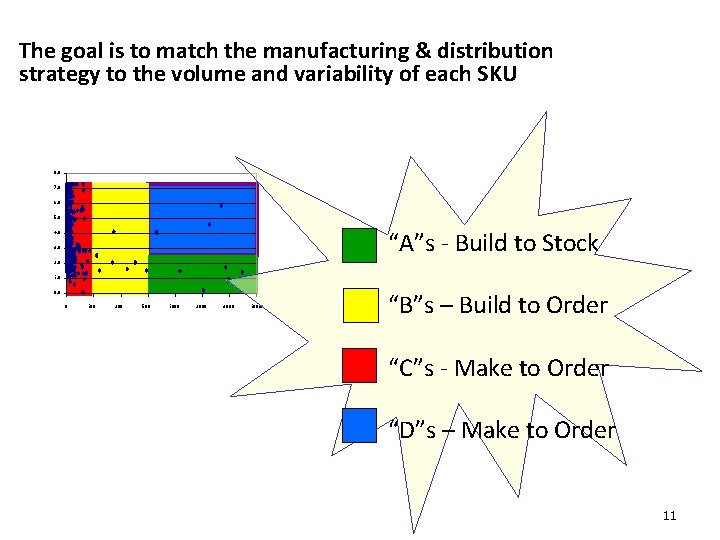
The goal is to match the manufacturing & distribution strategy to the volume and variability of each SKU 8. 0 7. 0 6. 0 5. 0 “A”s - Build to Stock 4. 0 3. 0 2. 0 1. 0 0 100 200 500 1000 2000 3000 10000 “B”s – Build to Order “C”s - Make to Order “D”s – Make to Order 11

MAQ Corporation Exercise 12

MAQ Corporation, a major producer of consumer electronics equipment, is currently faced with a rapidly growing product line and its associated inventory problems. MAQ’s President, Mary Semerod, has decided to initiate a program to analyze the company’s inventory requirements utilizing different inventory techniques. The first phase of the program consists of an ABC analysis of the companies product line (shown on following slide). Ms. Semerod has encountered difficulties in deciding on the appropriate criteria to use in the classification and in developing appropriate cutoff levels for each class of inventory. To solve her dilemma, Ms. Semerod has contracted the services of a logistics consulting firm to perform the inventory analysis 13

MAQ Corporation 1. If you were employed by the consulting firm, how would you construct your method of analysis? 2. What criteria would you use? 3. What would be the cutoff levels? Data 14

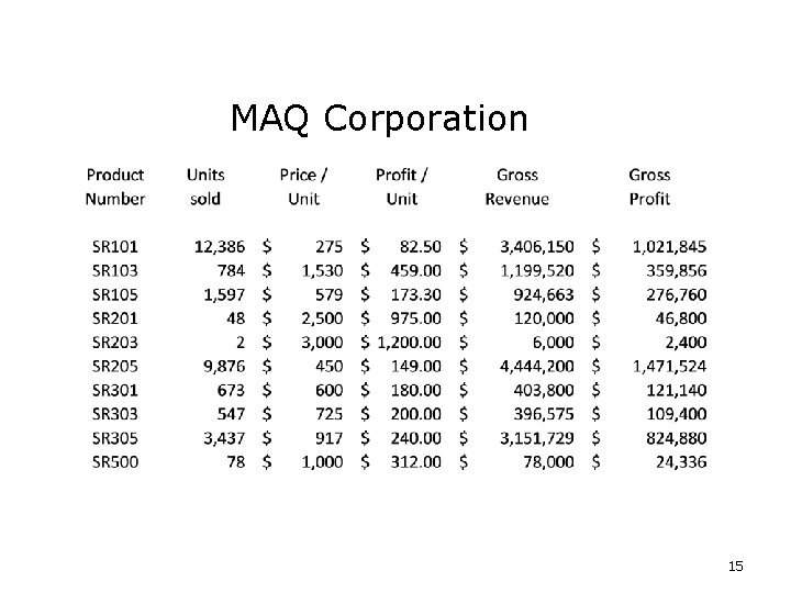
MAQ Corporation 15

Let’s take a break! When we return we take-up answering 2 questions: 1. How much should I order? 2. When should I order?

How much should I order? Total Inventory Cost includes = Holding Cost + Ordering Cost The Economic Order Quantity (EOQ) is the lowest total cost recognizing the trade off of: 1. As order size increases, holding cost increases 2. As order size increases, order cost decreases 17

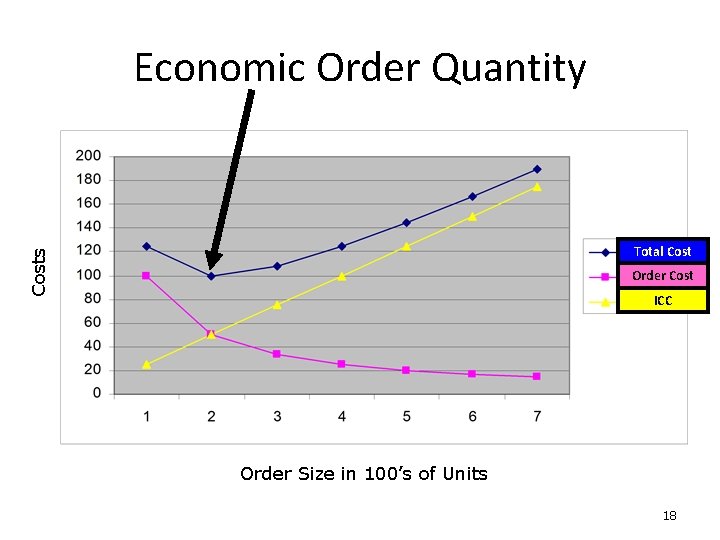
Economic Order Quantity Costs Total Cost Order Cost ICC Order Size in 100’s of Units 18

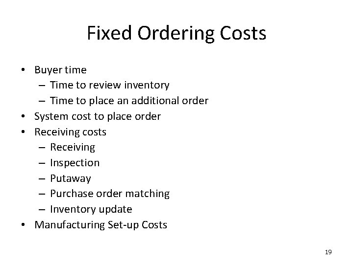
Fixed Ordering Costs • Buyer time – Time to review inventory – Time to place an additional order • System cost to place order • Receiving costs – Receiving – Inspection – Putaway – Purchase order matching – Inventory update • Manufacturing Set-up Costs 19

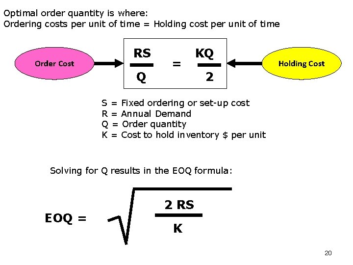
Optimal order quantity is where: Ordering costs per unit of time = Holding cost per unit of time Order Cost RS Q = KQ Holding Cost 2 S = Fixed ordering or set-up cost R = Annual Demand Q = Order quantity K = Cost to hold inventory $ per unit Solving for Q results in the EOQ formula: EOQ = 2 RS K 20

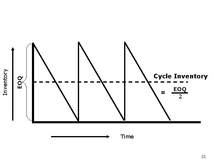
EOQ Inventory Cycle Inventory = EOQ 2 Time 21

EOQ Assumptions 1. Demand is known and constant 2. Order quantities are fixed at Q items per order 3. A fixed cost incurred on each order 4. Holding cost accrued per unit of time 5. Lead time is known and constant at 0 6. Initial inventory is 0 7. Infinite planning horizon 22

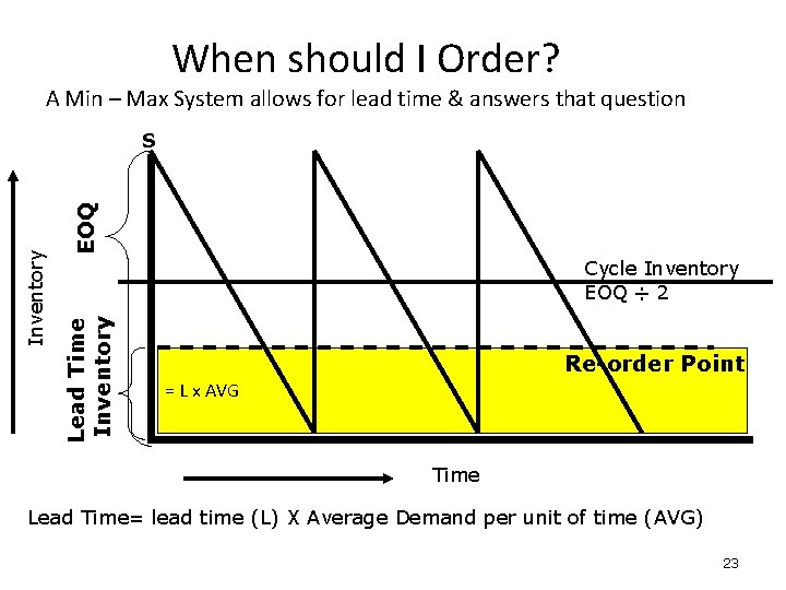
When should I Order? A Min – Max System allows for lead time & answers that question EOQ Cycle Inventory EOQ ÷ 2 Lead Time Inventory S Re-order Point = L x AVG Time Lead Time= lead time (L) X Average Demand per unit of time (AVG) 23

Nittany Fans 24

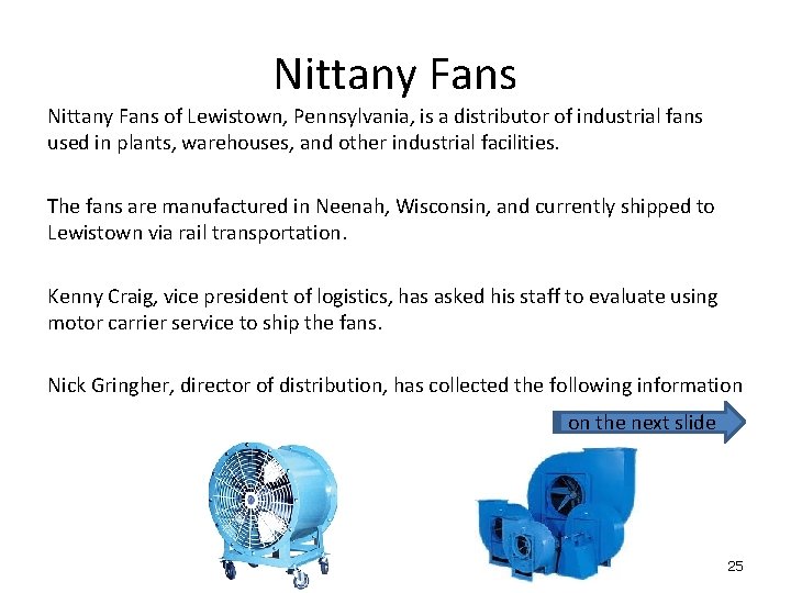
Nittany Fans of Lewistown, Pennsylvania, is a distributor of industrial fans used in plants, warehouses, and other industrial facilities. The fans are manufactured in Neenah, Wisconsin, and currently shipped to Lewistown via rail transportation. Kenny Craig, vice president of logistics, has asked his staff to evaluate using motor carrier service to ship the fans. Nick Gringher, director of distribution, has collected the following information on the next slide 25

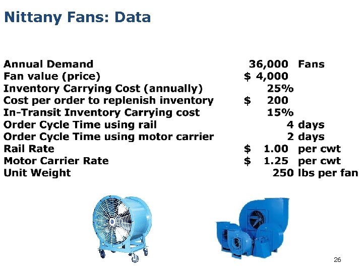
Nittany Fans: Data 26

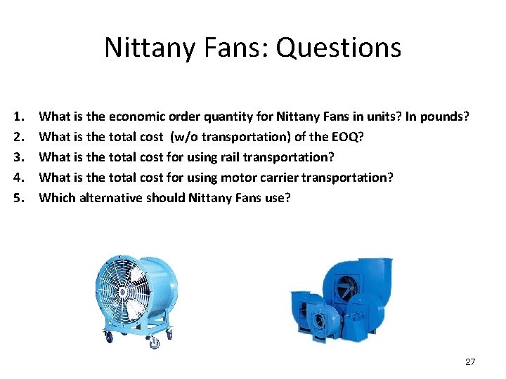
Nittany Fans: Questions 1. 2. 3. 4. 5. What is the economic order quantity for Nittany Fans in units? In pounds? What is the total cost (w/o transportation) of the EOQ? What is the total cost for using rail transportation? What is the total cost for using motor carrier transportation? Which alternative should Nittany Fans use? 27

Let’s take a break! When we return, we will take-up the question: 1. Do I have enough inventory? 2. How do I deal with uncertainty of demand? 3. How do I deal with uncertainty of supply?

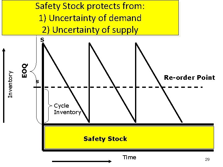
Safety Stock protects from: 1) Uncertainty of demand 2) Uncertainty of supply EOQ Inventory S Re-order Point s Cycle Inventory Safety Stock Time 29

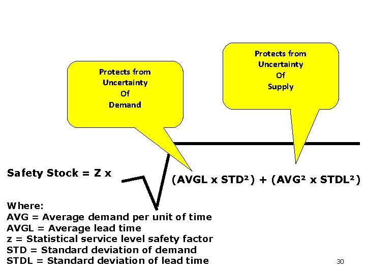
Protects from Uncertainty Of Supply Protects from Uncertainty Of Demand Safety Stock = Z x (AVGL x STD²) + (AVG² x STDL²) Where: AVG = Average demand per unit of time AVGL = Average lead time z = Statistical service level safety factor STD = Standard deviation of demand STDL = Standard deviation of lead time 30

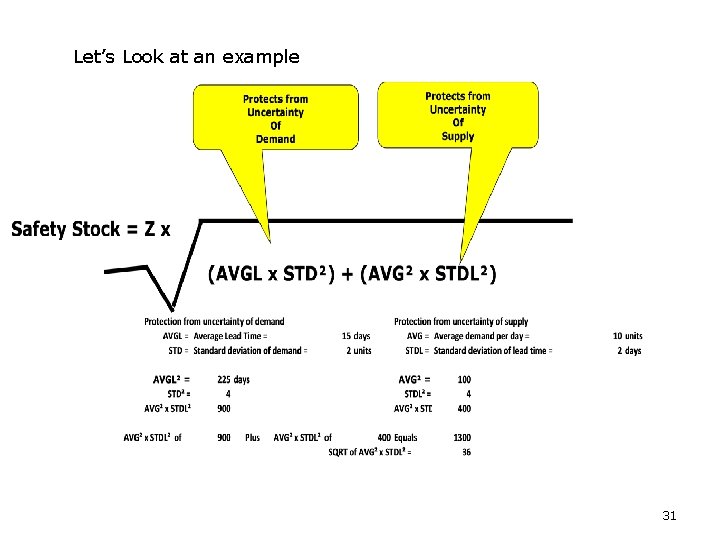
Let’s Look at an example 31

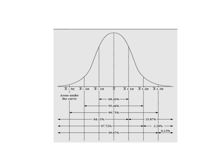
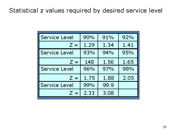
Statistical z values required by desired service level Service Level 90% 91% 92% 1. 29 1. 34 1. 41 93% 94% 95% Z = 148 Service Level 96% 1. 56 97% 1. 65 98% Z = 1. 75 Service Level 99% 1. 88 99. 9 2. 05 Z= Service Level Z= 2. 33 3. 08 33

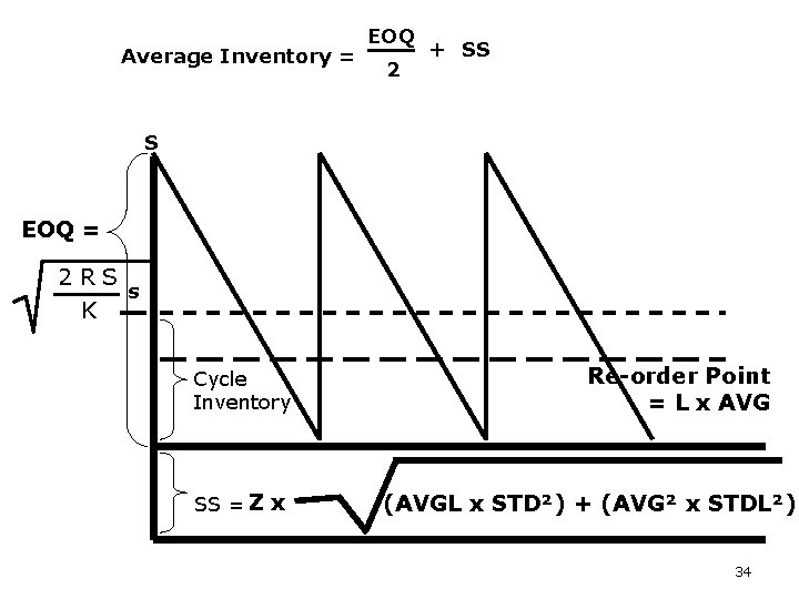
Average Inventory = EOQ 2 + SS S EOQ = 2 RS s K Cycle Inventory SS = Z x Re-order Point = L x AVG (AVGL x STD²) + (AVG² x STDL²) 34

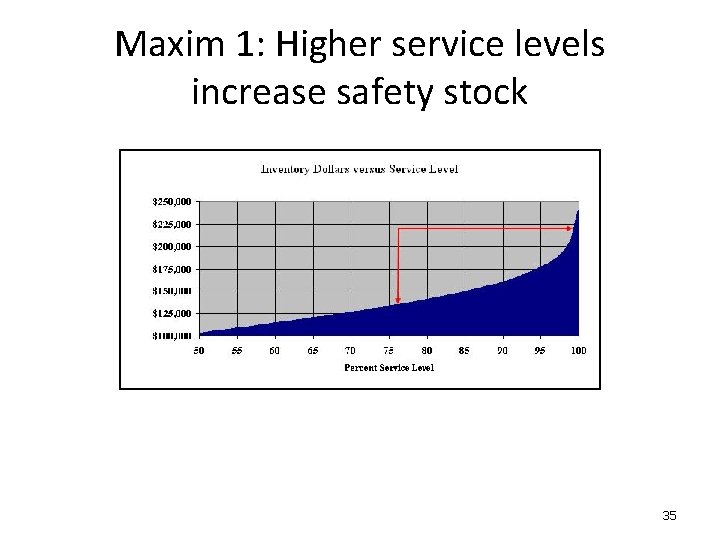
Maxim 1: Higher service levels increase safety stock 35

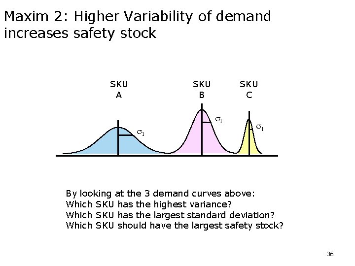
Maxim 2: Higher Variability of demand increases safety stock SKU A SKU B SKU C s 1 s 1 By looking at the 3 demand curves above: Which SKU has the highest variance? Which SKU has the largest standard deviation? Which SKU should have the largest safety stock? 36

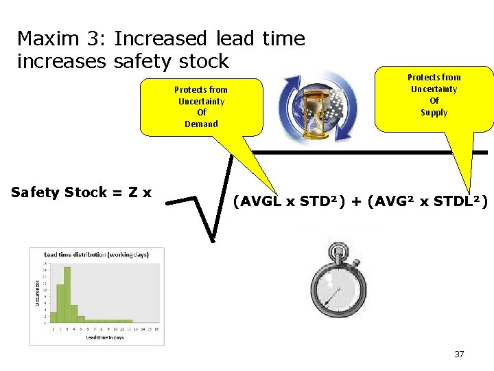
Maxim 3: Increased lead time increases safety stock Protects from Uncertainty Of Demand Safety Stock = Z x Protects from Uncertainty Of Supply (AVGL x STD²) + (AVG² x STDL²) 37

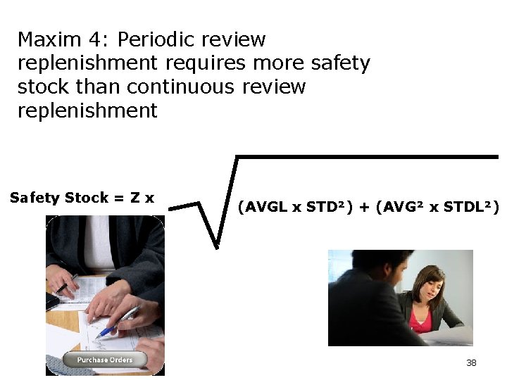
Maxim 4: Periodic review replenishment requires more safety stock than continuous review replenishment Safety Stock = Z x (AVGL x STD²) + (AVG² x STDL²) 38

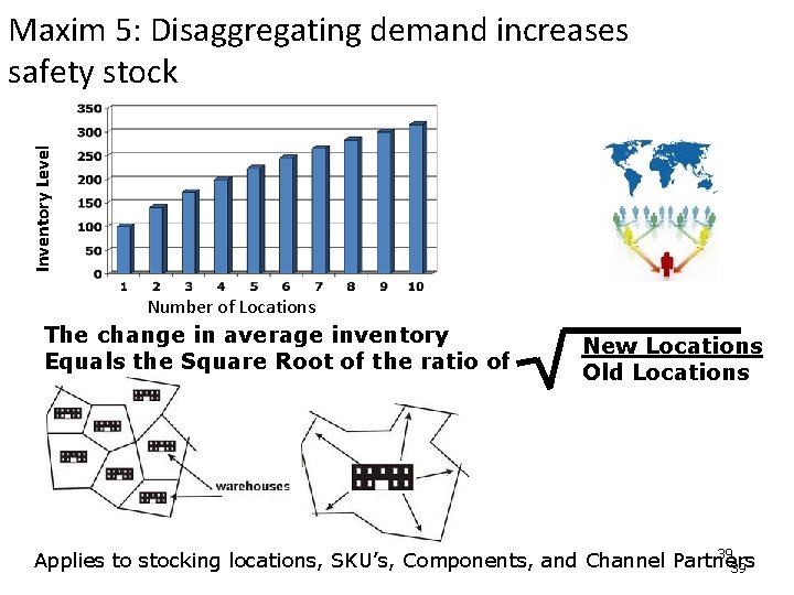
Inventory Level Maxim 5: Disaggregating demand increases safety stock Number of Locations The change in average inventory Equals the Square Root of the ratio of New Locations Old Locations 39 Applies to stocking locations, SKU’s, Components, and Channel Partners 39

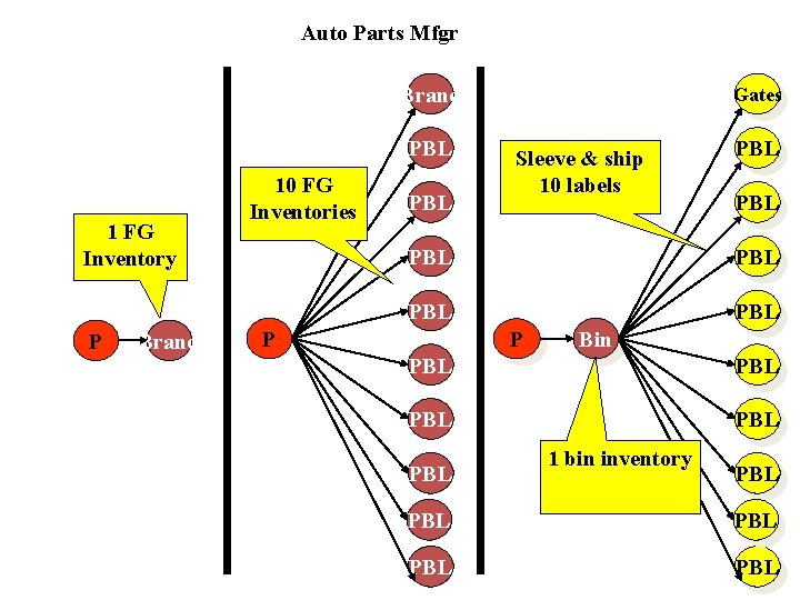
Auto Parts Mfgr Brand PBL 1 FG Inventory P GBrandes 10 FG Inventories PBL Gates Sleeve & ship 10 labels PBL PBL PBL P P Bin PBL PBL PBL 1 bin inventory PBL PBL 40 PBL

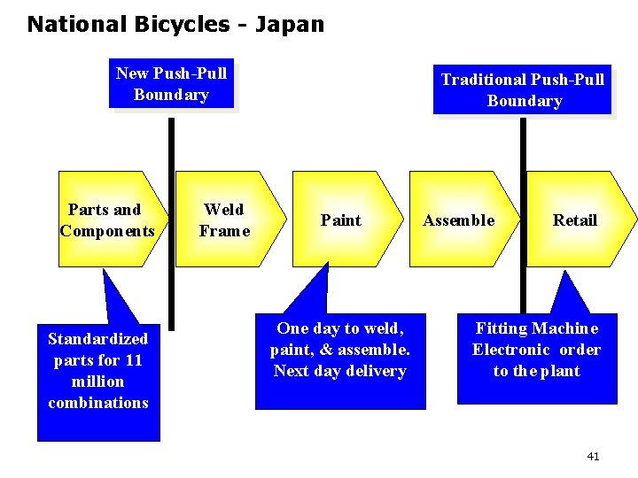
National Bicycles - Japan New Push-Pull Boundary Parts and Components Standardized parts for 11 million combinations Weld Frame Traditional Push-Pull Boundary Paint One day to weld, paint, & assemble. Next day delivery Assemble Retail Fitting Machine Electronic order to the plant 41

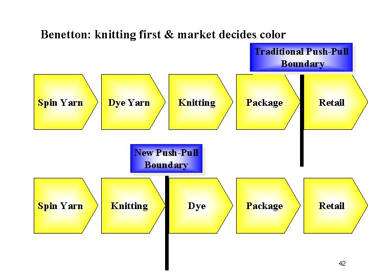
Benetton: knitting first & market decides color Traditional Push-Pull Boundary Spin Yarn Dye Yarn Knitting Package Retail New Push-Pull Boundary Spin Yarn Knitting Dye 42

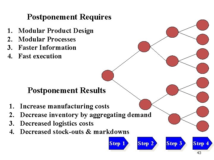
Postponement Requires 1. 2. 3. 4. Modular Product Design Modular Processes Faster Information Fast execution Postponement Results 1. 2. 3. 4. Increase manufacturing costs Decrease inventory by aggregating demand Decreased logistics costs Decreased stock-outs & markdowns Step 1 Step 2 Step 3 Step 4 43