Supply and Demand 2 1 Drawing on Chapter

Supply and Demand 2 -1

Drawing on Chapter 2 Mc. Graw-Hill/Irwin Graphics copyright © 2010 The Mc. Graw-Hill Companies, Inc. All rights reserved.

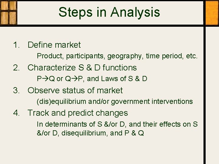
Steps in Analysis 1. Define market Product, participants, geography, time period, etc. 2. Characterize S & D functions P Q or Q P, and Laws of S & D 3. Observe status of market (dis)equilibrium and/or government interventions 4. Track and predict changes In determinants of S &/or D, and their effects on S &/or D, disequilibrium, and P & Q

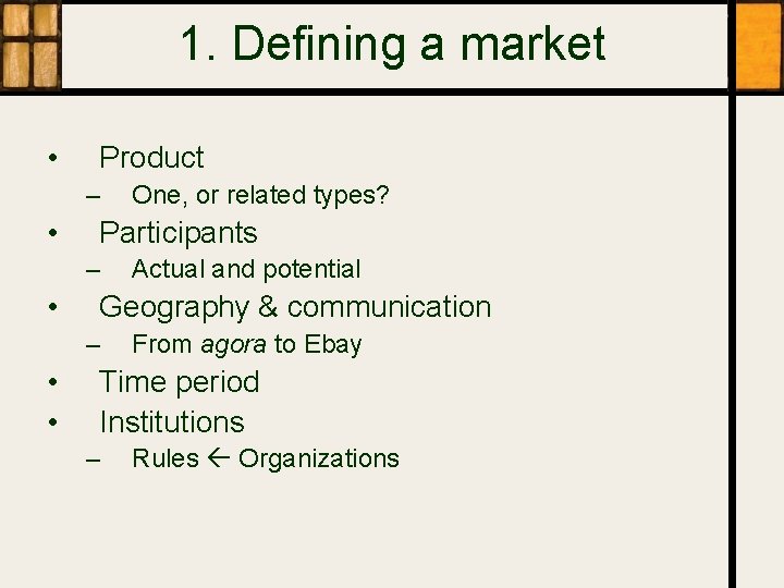
1. Defining a market • Product – • Participants – • Actual and potential Geography & communication – • • One, or related types? From agora to Ebay Time period Institutions – Rules Organizations

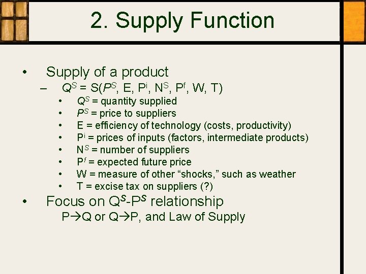
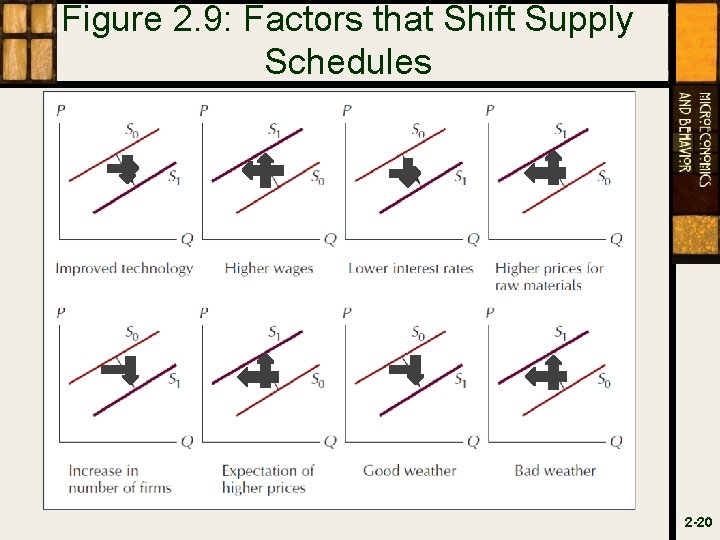
2. Supply Function • Supply of a product – QS = S(PS, E, Pi, NS, Pf, W, T) • • • QS = quantity supplied PS = price to suppliers E = efficiency of technology (costs, productivity) Pi = prices of inputs (factors, intermediate products) NS = number of suppliers Pf = expected future price W = measure of other “shocks, ” such as weather T = excise tax on suppliers (? ) Focus on QS-PS relationship P Q or Q P, and Law of Supply

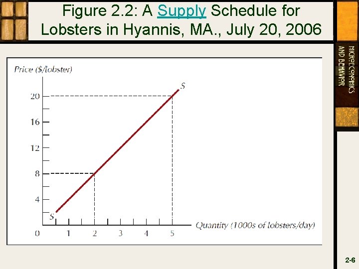
Figure 2. 2: A Supply Schedule for Lobsters in Hyannis, MA. , July 20, 2006 2 -6

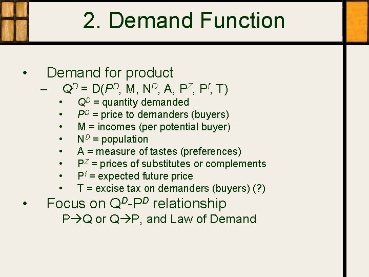
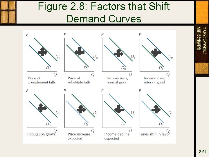
2. Demand Function • Demand for product – QD = D(PD, M, ND, A, PZ, Pf, T) • • • QD = quantity demanded PD = price to demanders (buyers) M = incomes (per potential buyer) ND = population A = measure of tastes (preferences) PZ = prices of substitutes or complements Pf = expected future price T = excise tax on demanders (buyers) (? ) Focus on QD-PD relationship P Q or Q P, and Law of Demand

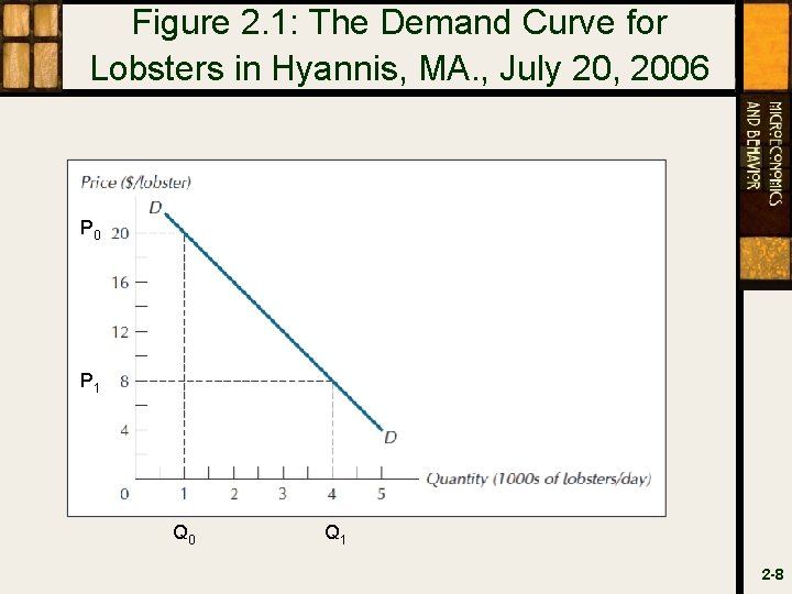
Figure 2. 1: The Demand Curve for Lobsters in Hyannis, MA. , July 20, 2006 P 0 P 1 Q 0 Q 1 2 -8

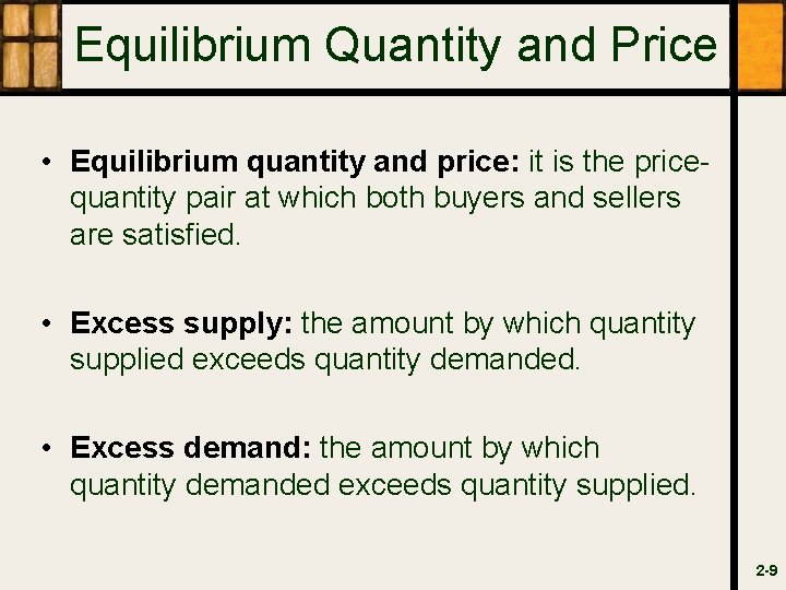
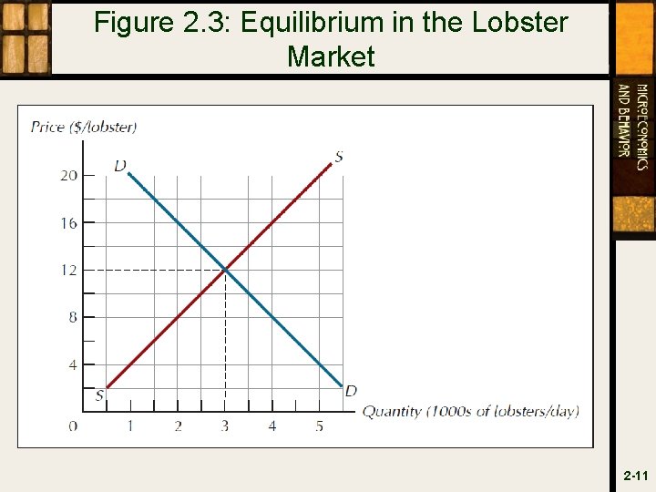
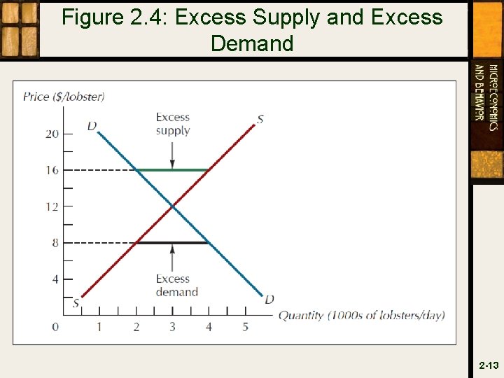
Equilibrium Quantity and Price • Equilibrium quantity and price: it is the pricequantity pair at which both buyers and sellers are satisfied. • Excess supply: the amount by which quantity supplied exceeds quantity demanded. • Excess demand: the amount by which quantity demanded exceeds quantity supplied. 2 -9

3. Status of Market: Equilibrium • • Attractor or destination, usually not current status Stable in short run

Figure 2. 3: Equilibrium in the Lobster Market 2 -11

3. Status of Market: Disequilibrium • Unstable – Excess supply or demand – Usually temporary unless … • Government controls – Price ceiling – Price support (such as a floor) – Production quota • Potential for welfare improvement

Figure 2. 4: Excess Supply and Excess Demand 2 -13

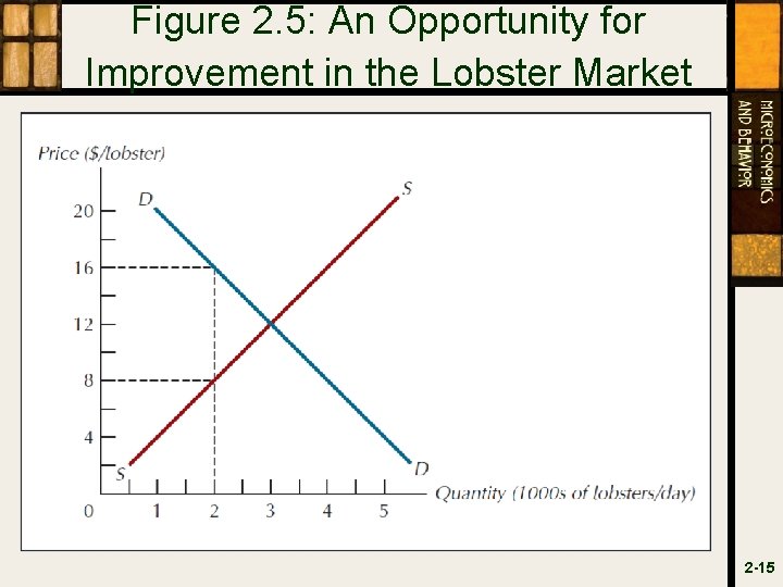
Figure 2. 5: An Opportunity for Improvement in the Lobster Market 2 -15

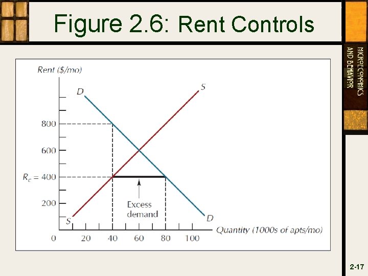
Figure 2. 6: Rent Controls 2 -17

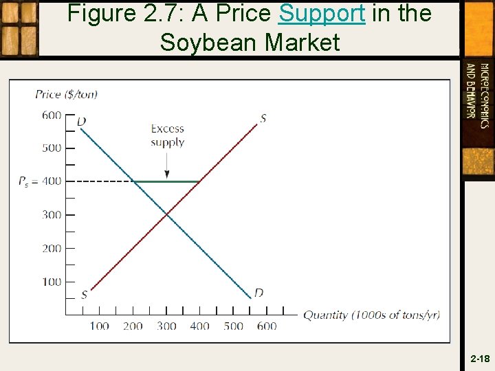
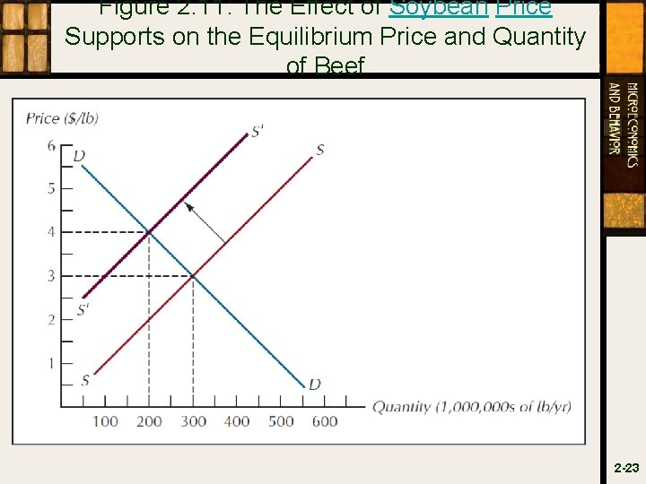
Figure 2. 7: A Price Support in the Soybean Market 2 -18

4. Track and Predict Changes • For each event, – – • Which does it affect: S &/or D? Which way? What type of disequilibrium? What changes in P & Q? Write and graph

Figure 2. 9: Factors that Shift Supply Schedules 2 -20

Figure 2. 8: Factors that Shift Demand Curves 2 -21

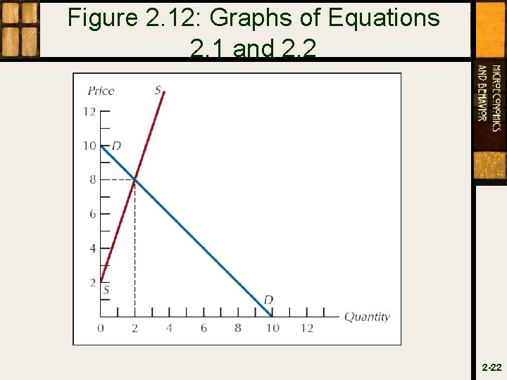
Figure 2. 12: Graphs of Equations 2. 1 and 2. 2 2 -22

Figure 2. 11: The Effect of Soybean Price Supports on the Equilibrium Price and Quantity of Beef 2 -23

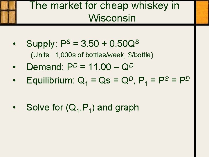
The market for cheap whiskey in Wisconsin • Supply: PS = 3. 50 + 0. 50 QS (Units: 1, 000 s of bottles/week, $/bottle) • • Demand: PD = 11. 00 – QD Equilibrium: Q 1 = Qs = QD, P 1 = PS = PD • Solve for (Q 1, P 1) and graph