Supervised Learning Methods knearestneighbors Decision trees Neural networks

Supervised Learning Methods • k-nearest-neighbors • Decision trees • Neural networks • Naïve Bayes • Support vector machines (SVM)

Support Vector Machines Chapter 18. 9 and the optional paper “Support vector machines” by M. Hearst, ed. , 1998 Acknowledgments: These slides combine and modify ones provided by Andrew Moore (CMU), Carla Gomes (Cornell), Mingyue Tan (UBC), Jerry Zhu (Wisconsin), Glenn Fung (Wisconsin), and Olvi Mangasarian (Wisconsin)
 Used For? • Classification • Regression and data-fitting")
What are Support Vector Machines (SVMs) Used For? • Classification • Regression and data-fitting • Supervised and unsupervised learning

Lake Mendota, Madison, WI • • Lake Mendota, Wisconsin Identify areas of land cover (land, ice, water, snow) in a scene Two methods: • • Scientist manually-derived Support Vector Machine (SVM) Classifier Expert Derived SVM cloud 45. 7% 58. 5% ice 60. 1% 80. 4% land 93. 6% 94. 0% snow 63. 5% 71. 6% water 84. 2% 89. 1% unclassified 45. 7% Courtesy of Steve Chien of NASA/JPL Visible Image Expert Labeled Expert Automated SVM Derived Ratio

Linear Classifiers x f y denotes +1 denotes -1 How would you classify this data?
 • Definition: A function that is a linear")
Linear Classifiers (aka Linear Discriminant Functions) • Definition: A function that is a linear combination of the components of the input (column vector) x: where w is the weight (column vector) and b is the bias • A 2 -classifier then uses the rule: Decide class c 1 if f(x) ≥ 0 and class c 2 if f(x) < 0 or, equivalently, decide c 1 if w. Tx ≥ -b and c 2 otherwise

w is the plane’s normal vector Planar decision surface in d dimensions is parameterized by (w, b) b is the distance from the origin w b
 = sign(w. T x")
Linear Classifiers x denotes +1 f y f(x, w, b) = sign(w. T x + b) denotes -1 How would you classify this data?
 = sign(w. T x")
Linear Classifiers x denotes +1 f y f(x, w, b) = sign(w. T x + b) denotes -1 How would you classify this data?
 = sign(w. T x")
Linear Classifiers x denotes +1 f y f(x, w, b) = sign(w. T x + b) denotes -1 How would you classify this data?
 = sign(w. T x")
Linear Classifiers x denotes +1 y f f(x, w, b) = sign(w. T x + b) denotes -1 Any of these would be fine … … but which is best?
 = sign(w.")
Classifier Margin x denotes +1 denotes -1 f y f(x, w, b) = sign(w. T x + b) Define the margin of a linear classifier as the width that the decision boundary could be expanded before hitting a data point
 = sign(w. T x")
Maximum Margin x denotes +1 f y f(x, w, b) = sign(w. T x + b) The maximum margin linear classifier is the linear classifier with the maximum margin denotes -1 This is the simplest kind of SVM (Called an LSVM) Linear SVM
 = sign(w. T x")
Maximum Margin x denotes +1 f y f(x, w, b) = sign(w. T x + b) The maximum margin linear classifier is the linear classifier with the maximum margin denotes -1 Support Vectors are those data points that the margin pushes against This is the simplest kind of SVM (Called an LSVM) Linear SVM

Why the Maximum Margin? 1. Intuitively this feels safest denotes +1 denotes -1 Support Vectors are those data points that the margin pushes against f(x, w, b) = sign(w. - b) 2. If we’ve made a small error inxthe location of the boundary (it’s been The maximum jolted in its perpendicular direction) this gives us leastmargin chance linear of causing a misclassification classifier is the 3. Robust to outlierslinear since the model is classifier immune to change/removal any with the, of um, non-support-vector data points maximum margin. 4. There’s some theory (using “VC is the simplest dimension”) that This is related to (but not of SVM the same as) thekind proposition that this is a good thing (Called an LSVM) 5. Empirically it works very well

Specifying a Line and Margin 1” + = ss a l t C one c i d z e r P “ Plus-Plane Classifier Boundary 1” = Minus-Plane ss a l t C one c i z red “P • How do we represent this mathematically? • … in d input dimensions? • An example x = (x 1, …, xd)T

Specifying a Line and Margin 1” + = Plus-Plane Classifier Boundary ss a l t C one c i d z e r P “ ss a l t C one c i z red 1 b= + 0 wx b= + wx b=-1 + wx Weight vector: w = (w 1 , …, wd)T “P Bias or threshold: b w. T x + b = +1 w. T x + b = -1 • Plus-plane = • Minus-plane = Classify as 1” = Minus-Plane The dot product is a scalar: x’s projection onto w +1 if w. T x + b ≥ 1 -1 if w. T x + b ≤ -1 ? if -1 < w T x + b < 1

Computing the Margin 1” + = ss a l t C one c i d z e r P “ w =1 b T x+ w =0 b T x+ 1 w =b T x+ w • Plus-plane = • Minus-plane = Margin (width) 1” = ss a l t C one c i z red “P How do we compute M in terms of w and b? w. T x + b = +1 w. T x + b = -1 Claim: The vector w is perpendicular to the Plus-Plane and the Minus-Plane

Computing the Margin 1” + + M = Margin x = s s la e C ct zon i d e “Pr 1” How do we compute w − x = s s la M in terms of w =1 C b e t + c on wx di z =0 e b r + and b? 1 “P wx =+b wx • • • Plus-plane = w. T x + b = +1 Minus-plane = w. T x + b = -1 The vector w is perpendicular to the Plus-Plane Let x− be any point on the Minus-Plane Let x+ be the closest Plus-Plane-point to x− Any location in dm: ; not R not necessarily a datapoint data point

Computing the Margin 1” + + M = Margin x = s s la e C ct zon i d e “Pr 1” How do we compute w − x = s s la M in terms of w =1 C b e t + c on wx di z =0 e b r + and b? 1 “P wx =+b wx • • • Plus-plane = w. T x + b = +1 Minus-plane = w. T x + b = -1 The vector w is perpendicular to the Plus-Plane Let x− be any point on the Minus-Plane Let x+ be the closest Plus-Plane-point to x− Claim: x+ = x− + λ w for some value of λ

Computing the Margin 1” + + M = Margin x = s s la e C − to x+ is ct zon The line from x i d e “Pr perpendicular to the do we compute 1” How w − x = s s planes a 1 l M in terms of w = C b e t + c on wx di z =0 e b r + and ? So to getbfrom x− to x+ “P -1 wx b= + wx • • • travel some distance in direction w Plus-plane = w. T x + b = +1 Minus-plane = w. T x + b = -1 The vector w is perpendicular to the Plus-Plane Let x− be any point on the Minus-Plane Let x+ be the closest Plus-Plane-point to x− Claim: x+ = x− + λ w for some value of λ Why?

Computing the Margin 1” + + M = Margin x = s s la e C ct zon i d e “Pr 1” w − x = s s la =1 C b t + c zone i 0 wx d = re +b -1 P x “ w b= + wx What we know: • w. T x+ + b = +1 • w T x - + b = -1 • x+ = x− + λ w • ||x+ - x− || = M

Computing the Margin 1” + + M = Margin x = s s la e C ct zon i d e “Pr 1” w − x = s s la =1 C b t + c zone i 0 wx d T (x− + λ w) = re w +b -1 P x “ w b= + wx What we know: • w. T x+ + b = +1 • w. T x− + b = -1 • x+ = x− + λ w • ||x+ - x− || = M It’s now easy to get M in terms of w and b +b=1 ⇒ w T x− + b + λ w T w = 1 ⇒ -1 + λ w T w = 1 ⇒

Computing the Margin 1” + + M = Margin = x = s s la e C ct zon i d e “Pr 1” w − x = s s la =1 C b t + c zone i 0 wx d = re M = ||x+ - x− || +b -1 P x “ w b= = || λw || + wx What we know: • w. T x+ + b = +1 • w. T x− + b = -1 • x+ = x− + λ w • ||x+ - x− || = M, margin size

Learning the Maximum Margin Classifier 1” + + M = Margin = x = s s la e C ct zon i d e “Pr 1” w − x = s s la =1 C b t + c zone i 0 wx d = re +b -1 P x “ w = +b wx Given a guess of w and b, we can 1. Compute whether all data points in the correct half-planes 2. Compute the margin So now we just need to write a program to search the space of w’s and b’s to find the widest margin that correctly classifies all the data points How?

SVM as Constrained Optimization • Unknowns: w, b • Objective function: maximize the margin: M = 2 / ||w|| • Equivalent to minimizing ||w|| or ||w||2 = w. Tw • N training points: (xk , yk), yk = +1 or -1 • Subject to each training point correctly classified, i. e. , N constraints subject to yk(w. Txk + b) ≥ 1 for all k This is a quadratic optimization problem (QP), which can be solved efficiently

Sec. 15. 1 Classification with SVMs Given a new point x, we can classify it by • Computing score: w. Tx + b • Deciding class based on whether < 0 or > 0 • If desired, can set confidence threshold t Score > t : yes Score < -t : no Else: don’t know -1 0 1

SVMs: More than Two Classes • SVMs can only handle two-class problems • k-class problem: Split the task into k binary tasks and learn k SVMs: • Class 1 vs. the rest (classes 2 — k) • Class 2 vs. the rest (classes 1, 3 — k) • … • Class k vs. the rest • Pick the class that puts the point farthest into its positive region

I vs II & III vs I & II from Statnikov et al.

SVMs: Non Linearly-Separable Data What if the data are not linearly separable?

SVMs: Non Linearly-Separable Data Two approaches: Allow a few points on the wrong side (slack variables) Map data to a higher dimensional space, and do linear classification there (kernel trick)

Non Linearly-Separable Data Approach 1: Allow a few points on the wrong side (slack variables) “Soft Margin Classification”

What Should We Do? denotes +1 denotes -1

What Should We Do? Idea: denotes +1 denotes -1 Minimize ||w||2 + C (# train errors) Tradeoff “penalty” parameter There’s a serious practical problem with this approach

What Should We Do? Idea: denotes +1 Minimize denotes -1 ||w||2 + C (# train errors) Tradeoff “penalty” parameter Can’t be expressed as a Quadratic There’s Programming problem. a serious practical problem with this approach So solving it may be too slow. (Also, doesn’t distinguish between disastrous errors and near misses)

What Should We Do? denotes +1 denotes -1 Minimize ||w||2 + C (distance of all “misclassified points” to their correct place)

Choosing C, the Penalty Factor Critical to choose a good value for the constant penalty parameter, C, because • C too big means very similar to LSVM because we have a high penalty for nonseparable points, and we may use many support vectors and overfit • C too small means we allow many misclassifications in the training data and we may underfit

Choosing C from Statnikov et al.

Learning Maximum Margin with Noise M= =1 b x+ w 0 b= + wx b=-1 + wx What should our optimization criterion be? Given guess of w, b, we can 1. Compute sum of distances of points to their correct zones 2. Compute the margin width Assume N examples, each (xk , yk) where yk = +1 / -1

Learning Maximum Margin with Noise ε 11 M= ε 2 =1 b x+ w 0 b= + wx b=-1 + wx ε 7 “slack variables” What should our optimization criterion be? Minimize Given guess of w, b, we can 1. Compute sum of distances of points to their correct zones 2. Compute the margin width Assume N examples, each (xk , yk) where yk = +1 / -1 How many constraints will we have? N What should they be? yk(w. Txk + b) ≥ 1 -εk for all k Note: εk = 0 for points in correct zone

Learning Maximum Margin dwith Noise = # input ε 2 =1 b x+ w 0 b= + wx b=-1 + wx ε 11 M = Given guessdimensions of w , b we can 1. Compute sum of distances of points to their correct Our original (noiseless data) QP had d +1 zones variables: w 1, w 2, … wd, and b 2. Compute the margin width e 7 Our new (noisy data) QP has d +1+N Assume R datapoints, each variables: w 1, w 2, … wd, b, ε k , ε 1 , … ε N (xk, yk) where yk = +/- 1 What should our optimization criterion be? Minimize How many constraints will we N = # examples have? N What should they be? w. Txk + b ≥ 1 - ε k if yk = +1 w. Txk + b ≤ -1+ε k if yk = -1

Learning Maximum Margin with Noise ε 2 =1 b x+ w 0 b= + wx b=-1 + wx ε 11 M = Given guess of w , ε 7 “slack variables” What should our optimization criterion be? Minimize b we can 1. Compute sum of distances of points to their correct zones 2. Compute the margin width Assume N examples, each (xk, yk) where yk = +1 / -1 How many constraints will we have? 2 N What should they be? w. Txk + b ≥ +1 - ε k if yk = +1 w. Txk + b ≤ -1 + ε k if yk = -1 ε k ≥ 0 for all k

Non Linearly-Separable Data Approach 2: Map data to a higher dimensional space, and then do linear classification there (called the kernel trick)

Suppose we’re in 1 Dimension What would SVMs do with this data? x=0

Suppose we’re in 1 Dimension x=0 Positive “plane” Negative “plane”

Harder 1 D Dataset: Not Linearly-Separable What can be done about this? x=0

Harder 1 D Dataset The Kernel Trick: Preprocess the data, mapping x into a higher dimensional space, z = Φ(x) For example: x=0 Here, Φ maps data from 1 D to 2 D In general, map from d-dimensional input space to k-dimensional z space

Harder 1 D Dataset The data is linearly separable in the new space, so use a linear SVM in the new space x=0 w. T Φ(x) + b = +1 The Kernel Trick: Preprocess the data, mapping x into a higher dimensional space, z = Φ(x)

Another Example Project examples into some higher dimensional space where the data is linearly separable, defined by z = Φ(x)

Another Example Project examples into some higher dimensional space where the CS 540, University of Wisconsin-Madison, C. R. Dyer data is linearly separable, defined by z = Φ(x)

Algorithm 1. Pick a Φ function 2. Map each training example, x, into the new higher-dimensional space using z = Φ(x) 3. Solve the optimization problem using the nonlinearly transformed training examples, z, to obtain a Linear SVM (with or without using the slack variable formulation) defined by w and b 4. Classify a test example, e, by computing: sign(w. T · Φ(e) + b)

Improving Efficiency • Time complexity of the original optimization formulation depends on the dimensionality, k, of z (k >> d) • We can convert the optimization problem into an equivalent form, called the Dual Form, with time complexity O(N 3) that depends on N, the number of training examples, not k • Dual Form will also allow us to rewrite the mapping functions in Φ in terms of “kernel functions” instead

Dual Optimization Problem Maximize where subject to these constraints: Then define: Then classify with: f(x, w, b) = sign(w. Tx - b) N examples: (xk, yk) where yk = +1 / -1

Dual Optimization Problem Dot product of two examples Maximize where subject to these constraints: Then define: New variables; Examples with α k > 0 will be the support vectors Then classify with: f(x, w, b) = sign(w. Tx - b) N examples: (xk, yk) where yk = +1 / -1

Algorithm • Compute N x N matrix Q by computing yi yj (xi. T xj) between all pairs of training examples • Solve the optimization problem to compute αi for i = 1, …, N • Each non-zero αi indicates that example xi is a support vector • Compute w and b • Then classify test example x with: f(x) = sign(w. T x – b)
 Maximize where Subject to these constraints: Then define: Then")
Dual Optimization Problem (After Mapping) Maximize where Subject to these constraints: Then define: Then classify with: f(x, w, b) = sign(w. T Φ(x) - b) N examples: (xk, yk) where yk = +1 / -1 Copyright © 2001, 2003, Andrew W. Moore
 Maximize Subject to these constraints: where N 2 dot")
Dual Optimizzation Problem (After Mapping) Maximize Subject to these constraints: where N 2 dot products to compute this matrix Then define: Then classify with: f(x, w, b) = sign(w. T Φ(x) - b) N examples: (xk, yk) where yk = +1 / -1 Copyright © 2001, 2003, Andrew W. Moore

• Dual formulation of the optimization problem depends on the input data only in dot products of the form: Φ(xi)T · Φ(xj) where xi and xj are two examples • We can compute these dot products efficiently for certain types of Φ’s where K(xi, xj) = Φ(xi)T · Φ(xj) • Example: Φ(xi)T · Φ(xj) = (xi. T · xj)2 = K(xi , xj ) • Since the data only appears as dot products, we do not need to map the data to higher dimensional space (using Φ(x) ) because we can use the kernel function K instead
, is a dot product in some feature")
Kernel Functions • A kernel, K(xi, xj), is a dot product in some feature space • A kernel function is a function that can be applied to pairs of input examples to evaluate dot products in some corresponding (possibly infinite dimensional) feature space • We do not need to compute Φ explicitly
 is: s")
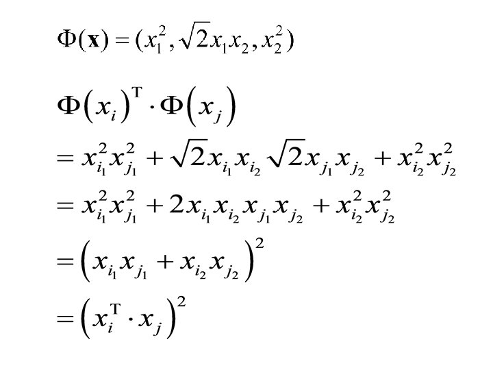
What’s Special about a Kernel? • Say 1 example (in 2 D) is: s = (s 1, s 2) • We decide to use a particular mapping into 6 D space: Φ(s)T = (s 12, s 22, √ 2 s 1 s 2, s 1, s 2, 1) • Let another example be t = (t 1, t 2) • Then, Φ(s)T Φ(t) = s 12 t 12 + s 22 t 22 + 2 s 1 s 2 t 1 t 2 + s 1 t 1 + s 2 t 2 + 1 = (s 1 t 1 + s 2 t 2 + 1)2 = (s. T t +1)2 • So, define the kernel function to be K(s, t) = (s. T t +1)2 = Φ(s)T Φ(t) • We save computation by using kernel K
 = xi. T")
Some Commonly Used Kernels • • Linear kernel: K(xi , xj) = xi. T xj Quadratic kernel: K(xi , xj) = (xi. T xj +1)2 Polynomial of degree d kernel: K(xi , xj) = (xi. T xj +1)d Radial-Basis Function (Gaussian) kernel: K(xi , xj) = exp(−||xi -xj ||2 / σ2) • Many possible kernels; picking a good one is tricky • Hacking with SVMs: create various kernels, hope their space Φ is meaningful, plug them into SVM, pick one with good classification accuracy • Kernel usually combined with slack variables because no guarantee of linear separability in new space

Algorithm • Compute N x N matrix Q by computing yi yj K(xi , xj ) between all pairs of training points • Solve optimization problem to compute αi for i = 1, …, N • Each non-zero αi indicates that example xi is a support vector • Compute w and b • Classify test example x using: f(x) = sign(w. T x – b)

Applications of SVMs n n n Bioinformatics Machine Vision Text Categorization Ranking (e. g. , Google searches) Handwritten Character Recognition Time series analysis Lots of very successful applications!

Handwritten Digit Recognition

Example Application: The Federalist Papers Dispute • Written in 1787 -1788 by Alexander Hamilton, John Jay, and James Madison to persuade the citizens of New York to ratify the U. S. Constitution • Papers consisted of short essays, 900 to 3500 words in length • Authorship of 12 of those papers have been in dispute ( Madison or Hamilton); these papers are referred to as the disputed Federalist papers

Description of the Data • For every paper: • Computed relative frequencies of 70 words that Mosteller -Wallace identified as good candidates for authorattribution studies • Each document is represented as a vector containing the 70 real numbers corresponding to the 70 word “Bag of frequencies • The dataset consists of 118 papers: • 50 Madison papers • 56 Hamilton papers • 12 disputed papers words”

70 -Word Dictionary

Feature Selection for Classifying the Disputed Federalist Papers • Apply the SVM algorithm for feature selection to: • Train on the 106 Federalist papers with known authors • Find a classification hyperplane (LSVM) that uses as few words as possible • Use the hyperplane to classify the 12 disputed papers

Hyperplane Classifier Using 3 Words • A hyperplane depending on three words was found: 0. 537 to + 24. 663 upon + 2. 953 would = 66. 616 • All disputed papers ended up on the Madison side of the plane

Results: 3 D Plot of Hyperplane

Summary • Learning linear functions • Pick separating hyperplane that maximizes margin • Separating plane defined in terms of support vectors (small number of training examples) only • Learning non-linear functions • Project examples into a higher dimensional space • Use kernel functions for efficiency • Generally avoids overfitting problem • Global optimization method; no local optima • Can be expensive to apply, especially for multi-class problems • Biggest Drawback: The choice of kernel function • There is no “set-in-stone” theory for choosing a kernel function for any given problem • Once a kernel function is chosen, there is only ONE modifiable parameter, the error penalty C

Software • A list of SVM implementations can be found at http: //www. kernel-machines. org/software. html • Some implementations (such as LIBSVM) can handle multi-classification • SVMLight is one of the earliest and most frequently used implementations of SVMs • Several Matlab toolboxes for SVMs are available
- Slides: 73