Supervised Learning in Neural Networks Learning when all

Supervised Learning in Neural Networks Learning when all the correct answers are available.

Remembering -vs- Learning • Remember: Store a given piece of information such that it can be retrieved and reused in the future in the same (or very similar) way that it was used earlier. • Learn: Extract useful generalizations (or specializations) from information such that, in the future, it may be: – Applied to new (previously unseen) situations – More effectively applied to previously-seen cases

Supervised Learning • Generalizing (and specializing) useful knowledge from data items, each of which contains both a situation (context) and the proper response (action) for that situation. • In an educational setting, the teacher provides a problem and THE CORRECT ANSWER. • In Reinforcement Learning (RL) the teacher only responds “Right” or “Wrong”.

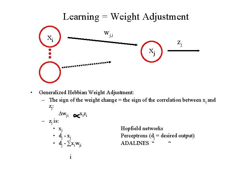
Learning = Weight Adjustment wj, i xi xj • zj Generalized Hebbian Weight Adjustment: – The sign of the weight change = the sign of the correlation between xi and zj: ∆wji xizi – zj is: • xj Hopfield networks • dj - xj Perceptrons (dj = desired output) • dj - ∑xiwji ADALINES “ “ i

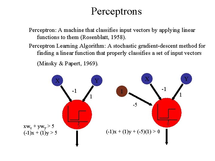
Perceptrons Perceptron: A machine that classifies input vectors by applying linear functions to them (Rosenblatt, 1958). Perceptron Learning Algorithm: A stochastic gradient-descent method for finding a linear function that properly classifies a set of input vectors (Minsky & Papert, 1969). X X Y -1 1 1 -5 xwx + ywy > 5 (-1)x + (1)y > 5 0 5 (-1)x + (1)y + (-5)(1) > 0

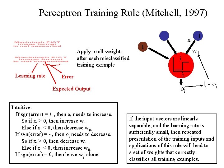
Perceptron Training Rule (Mitchell, 1997) Apply to all weights after each misclassified training example Learning rate Error Expected Output Intuitive: If sgn(error) = + , then oi needs to increase. So if xj > 0, then increase wij. Else if xj < 0, then decrease wij. If sgn(error) = - , then oi needs to decrease. So if xj > 0, then decrease wij. Else if xj < 0, then increase wij. If sgn(error) = 0, then leave wij alone. xj 1 j wij i 0 oi t i - oi If the input vectors are linearly separable, and the learning rate is sufficiently small, then repeated presentation of the training inputs and applications of this rule will lead to a set of weights that correctly classifies all training examples.

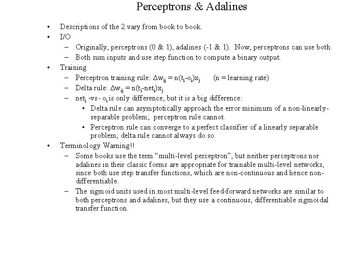
Perceptrons & Adalines • • Descriptions of the 2 vary from book to book. I/O – Originally, perceptrons (0 & 1), adalines (-1 & 1). Now, perceptrons can use both. – Both sum inputs and use step function to compute a binary output. Training – Perceptron training rule: ∆wij = n(ti-oi)xj (n = learning rate) – Delta rule: ∆wij = n(ti-neti)xj – neti -vs- oi is only difference, but it is a big difference: • Delta rule can asymptotically approach the error minimum of a non-linearlyseparable problem; perceptron rule cannot. • Perceptron rule can converge to a perfect classifier of a linearly separable problem; delta rule cannot always do so. Terminology Warning!! – Some books use the term “multi-level perceptron”, but neither perceptrons nor adalines in their classic forms are appropriate for trainable multi-level networks, since both use step transfer functions, which are non-continuous and hence nondifferentiable. – The sigmoid units used in most multi-level feed-forward networks are similar to both perceptrons and adalines, but they use a continuous, differentiable sigmoidal transfer function.

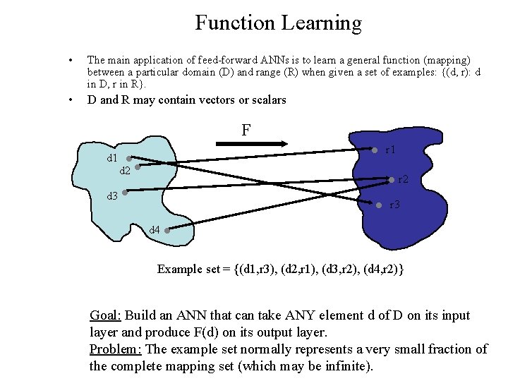
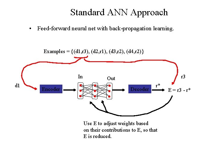
Function Learning • The main application of feed-forward ANNs is to learn a general function (mapping) between a particular domain (D) and range (R) when given a set of examples: {(d, r): d in D, r in R}. • D and R may contain vectors or scalars F r 1 d 2 r 2 d 3 r 3 d 4 Example set = {(d 1, r 3), (d 2, r 1), (d 3, r 2), (d 4, r 2)} Goal: Build an ANN that can take ANY element d of D on its input layer and produce F(d) on its output layer. Problem: The example set normally represents a very small fraction of the complete mapping set (which may be infinite).

Standard ANN Approach • Feed-forward neural net with back-propagation learning. Examples = {(d 1, r 3), (d 2, r 1), (d 3, r 2), (d 4, r 2)} In d 1 Encoder r 3 Out Decoder r* Use E to adjust weights based on their contributions to E, so that E is reduced. E = r 3 - r*

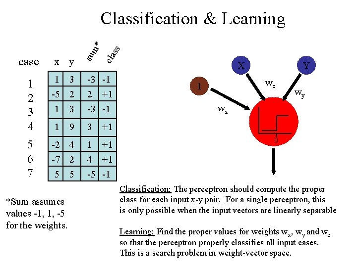
x y 1 2 3 4 1 3 -5 2 1 3 5 6 7 -2 4 -7 2 5 5 1 *Sum assumes values -1, 1, -5 for the weights. 9 ss cla case sum * Classification & Learning -3 -1 2 +1 -3 -1 3 X Y wx 1 wy wz +1 1 +1 4 +1 -5 -1 0 Classification: The perceptron should compute the proper class for each input x-y pair. For a single perceptron, this is only possible when the input vectors are linearly separable Learning: Find the proper values for weights wx, wy and wz so that the perceptron properly classifies all input cases. This is a search problem in weight-vector space.

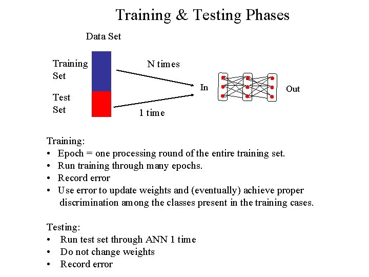
Training & Testing Phases Data Set Training Set Test Set N times In Out 1 time Training: • Epoch = one processing round of the entire training set. • Run training through many epochs. • Record error • Use error to update weights and (eventually) achieve proper discrimination among the classes present in the training cases. Testing: • Run test set through ANN 1 time • Do not change weights • Record error

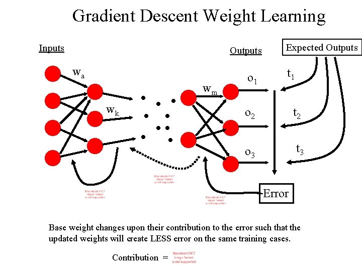
Gradient Descent Weight Learning Inputs Outputs wa wm wk o 1 Expected Outputs t 1 o 2 t 2 o 3 t 3 Error Base weight changes upon their contribution to the error such that the updated weights will create LESS error on the same training cases. Contribution =

Gradient Descent E w 32 w 31 = Gradient of E w. r. t. the weight vector

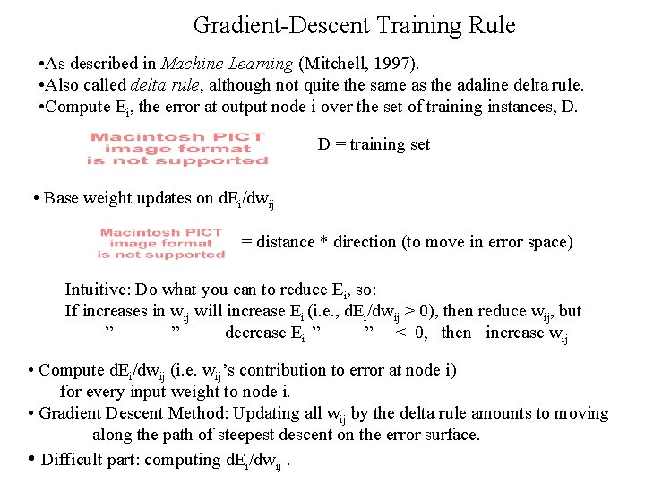
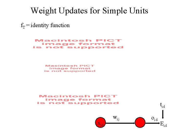
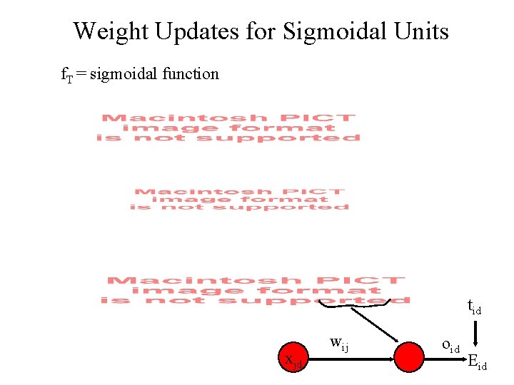
Gradient-Descent Training Rule • As described in Machine Learning (Mitchell, 1997). • Also called delta rule, although not quite the same as the adaline delta rule. • Compute Ei, the error at output node i over the set of training instances, D. D = training set • Base weight updates on d. Ei/dwij = distance * direction (to move in error space) Intuitive: Do what you can to reduce Ei, so: If increases in wij will increase Ei (i. e. , d. Ei/dwij > 0), then reduce wij, but ” ” decrease Ei ” ” < 0, then increase wij • Compute d. Ei/dwij (i. e. wij’s contribution to error at node i) for every input weight to node i. • Gradient Descent Method: Updating all wij by the delta rule amounts to moving along the path of steepest descent on the error surface. • Difficult part: computing d. Ei/dwij.

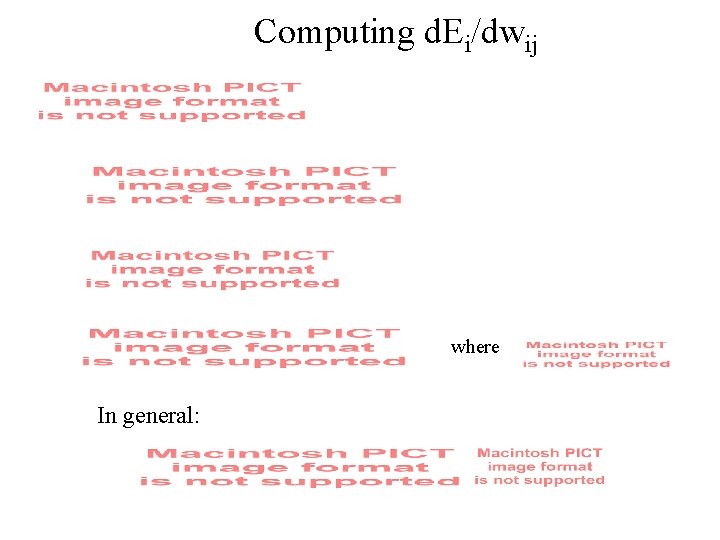
Computing d. Ei/dwij where In general:

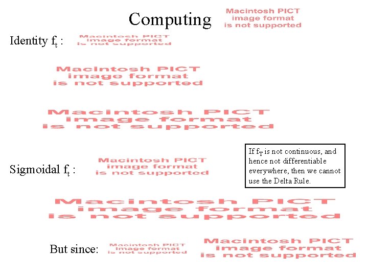
Computing Identity ft : Sigmoidal ft : But since: If f. T is not continuous, and hence not differentiable everywhere, then we cannot use the Delta Rule.

Weight Updates for Simple Units f. T = identity function tid xjd wij oid Eid

Weight Updates for Sigmoidal Units f. T = sigmoidal function tid xjd wij oid Eid

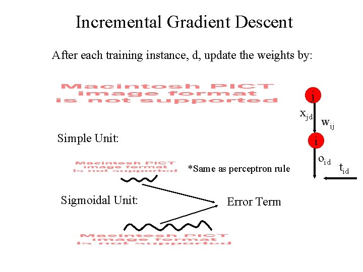
Incremental Gradient Descent After each training instance, d, update the weights by: j xjd Simple Unit: i *Same as perceptron rule Sigmoidal Unit: wij Error Term oid tid

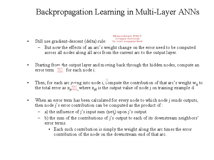
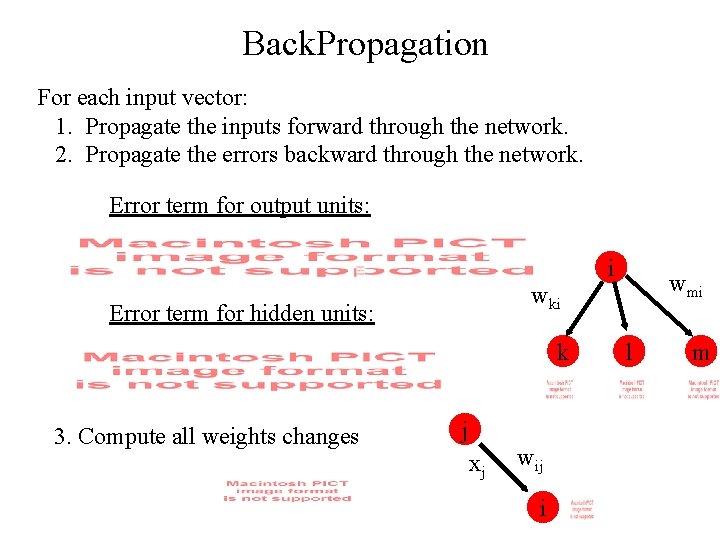
Backpropagation Learning in Multi-Layer ANNs • Still use gradient-descent (delta) rule: – But now the effects of an arc’s weight change on the error need to be computed across all nodes along all arcs from the current arc to the output layer. • Starting from the output layer and moving back through the hidden nodes, compute an error term for each node i. • Then, for each arc going into node i, compute the contribution of that arc’s weight wij to the total error as xjd , where xjd is the output value of node j on training example d. • When an error term has been calculated for every node to which node j sends outputs, then node j’s error contribution can be computed as the product of : – a) the influence of j’s input sum (netj) upon j’s output. – b) the sum of the contributions of j’s output to each of its downstream neighbors’ error terms. • Each such contribution is simply the weight along the arc times the error contribution of the node on the downstream end of that arc.

Back. Propagation For each input vector: 1. Propagate the inputs forward through the network. 2. Propagate the errors backward through the network. Error term for output units: i Error term for hidden units: k 3. Compute all weights changes wmi wki j xj wij i l m

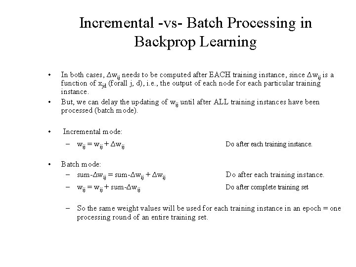
Incremental -vs- Batch Processing in Backprop Learning • • • In both cases, ∆wij needs to be computed after EACH training instance, since ∆wij is a function of xjd (forall j, d), i. e. , the output of each node for each particular training instance. But, we can delay the updating of wij until after ALL training instances have been processed (batch mode). Incremental mode: – wij = wij + ∆wij • Batch mode: – sum-∆wij = sum-∆wij + ∆wij – wij = wij + sum-∆wij Do after each training instance. Do after complete training set – So the same weight values will be used for each training instance in an epoch = one processing round of an entire training set.

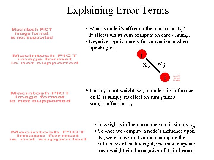
Explaining Error Terms • What is node i’s effect on the total error, Ed? It affects via its sum of inputs on case d, sumid. • Negative sign is merely for convenience when updating wij. j xjd wij i • For any input weight, wij, to node i, its influence on Ed is simply its effect on sumid times sumid’s effect on Ed. • A weight’s influence on the sum is simply xjd • So once we compute a node’s influence upon Ed, we can use that value to compute the influences of each weight, and thus to update each weight via the negative of its influence.

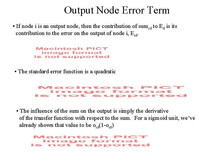
Output Node Error Term • If node i is an output node, then the contribution of sumid to Ed is its contribution to the error on the output of node i, Eid. • The standard error function is a quadratic • The influence of the sum on the output is simply the derivative of the transfer function with respect to the sum. For a sigmoid unit, we’ve already shown that value to be oid(1 -oid)

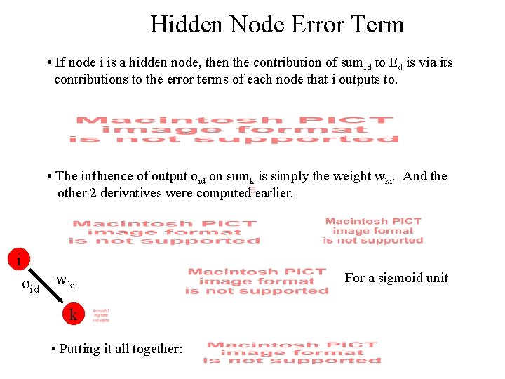
Hidden Node Error Term • If node i is a hidden node, then the contribution of sumid to Ed is via its contributions to the error terms of each node that i outputs to. • The influence of output oid on sumk is simply the weight wki. And the other 2 derivatives were computed earlier. i oid wki k • Putting it all together: For a sigmoid unit

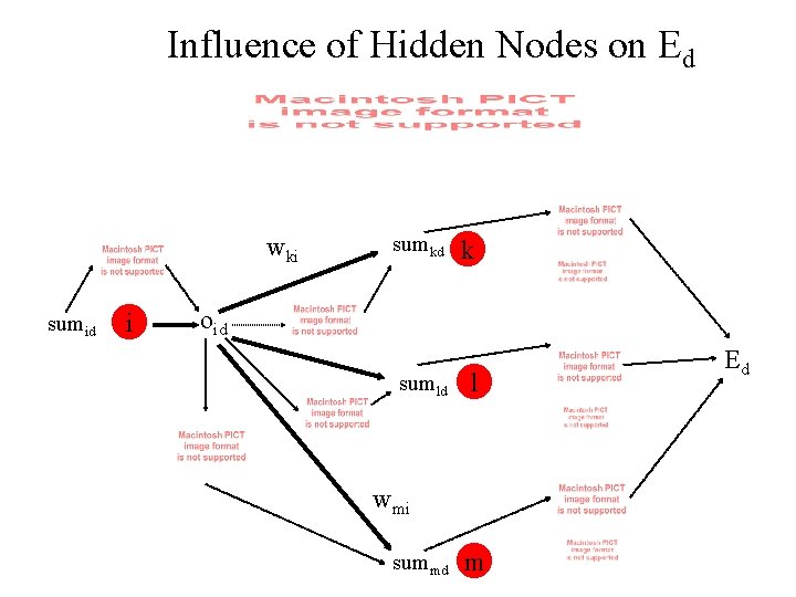
Influence of Hidden Nodes on Ed wki sumid i sumkd k oid sumld l wmi summd m Ed

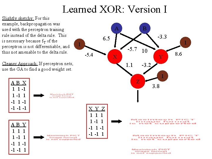
Learned XOR: Version I Slightly sketchy: For this example, backpropagation was used with the perceptron training rule instead of the delta rule. This is necessary because f. T of the perceptron is not differentiable, and thus not amenable to the delta rule. A AB Y 1 1 -1 -1 -1 1 -3. 3 6. 5 1 -5. 4 Cleaner Approach: If perceptron nets, use the GA to find a good weight set. AB X 1 1 -1 -1 -1 -1 B X -5. 7 10 1. 1 -3. 2 Z X Y Z 1 1 -1 -1 -1 1 Y 1 3. 8 1 8. 6

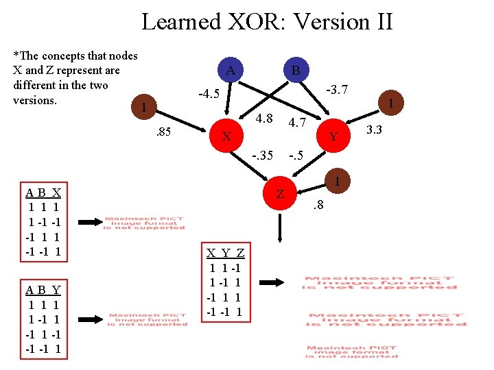
Learned XOR: Version II *The concepts that nodes X and Z represent are different in the two versions. A B -3. 7 -4. 5 1. 85 4. 8 4. 7 X -. 35 AB X 1 1 -1 -1 -1 1 AB Y 1 1 -1 -1 -1 1 -. 5 Z X Y Z 1 1 -1 -1 1 Y 1. 8 1 3. 3

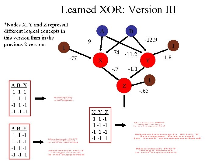
Learned XOR: Version III *Nodes X, Y and Z represent different logical concepts in this version than in the previous 2 versions A B -12. 9 9 1 -77 X 74 -11. 2 -. 7 AB X 1 1 -1 -1 -1 AB Y 1 1 -1 -1 -1. 1 Z X Y Z 1 1 -1 -1 1 Y 1 -. 65 1 -1. 8

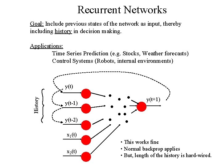
Recurrent Networks Goal: Include previous states of the network as input, thereby including history in decision making. Applications: Time Series Prediction (e. g. Stocks, Weather forecasts) Control Systems (Robots, internal environments) History y(t) y(t-1) y(t+1) y(t-2) x 1(t) x 2(t) • This works fine • Normal backprop applies • But, length of the history is hard-wired.

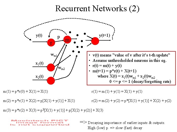
Recurrent Networks (2) y(t) p r m wm 1 x 1(t) y(t+1) wm 2 x 2(t) • • v(t) means ”value of v after it’s t-th update” Assume unthresholded neurons in this eg. r(t) = m(t) + y(t) m(t+1) = p*r(t) + X(t+1) where X(t) = x 1(t)wm 1 + x 2(t)wm 2 0 <= p <= 1 (decay/forgetting rate) m(1) = p*r(0) + X(1) = X(1) r(1) = m(1) + y(1) = X(1) + y(1) m(2) = p*r(1) + X(2) = p[X(1) + y(1)] + X(1) r(2) = m(2) + y(2) = p*[X(1) + y(1)] + X(2) + y(2) m(3) = p*r(2) + X(3) = p 2[X(1) + y(1)] + p[X(2) + y(2)] + X(3) => Decaying importance of earlier inputs & outputs. High (low) p => slow (fast) decay

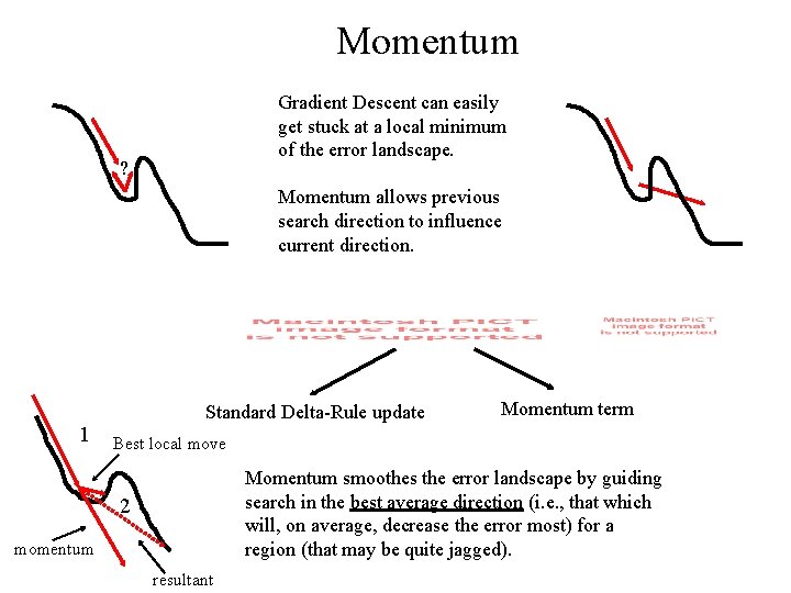
Momentum Gradient Descent can easily get stuck at a local minimum of the error landscape. ? Momentum allows previous search direction to influence current direction. 1 Standard Delta-Rule update Momentum term Best local move Momentum smoothes the error landscape by guiding search in the best average direction (i. e. , that which will, on average, decrease the error most) for a region (that may be quite jagged). 2 momentum resultant

Design Issues for Learning ANNs • Initial Weights – Random -vs- Biased – Width of init range • Typically: [-1 1] or [-0. 5] • Too wide => large weights will drive many sigmoids to saturation => all output 1 => takes a lot of training to undo. • Frequency of Weight Updates – Incremental - after each input. • In some cases, all training instances are not available at the same time, so the ANN must improve on-line. • Sensitive to presentation order. – Batch - after each epoch. • Uses less computation time • Insensitive to presentation order

Design Issues (2) • Learning Rate – Low value => slow learning – High value => faster learning, but oscillation due to overshoot – Typical range: [0. 1 0. 9] - Very problem specific! – Dynamic learning rate (many heuristics): • Gradually decrease over the epochs • Increase (decrease) whenever performance improves (worsens) • Use 2 nd deriv of error function – d 2 E/dw 2 high => changing d. E/dw => rough landscape => lower learning rate – d 2 E/dw 2 low => d. E/dw ~ constant => smooth landscape => raise learning rate • Length of Training Period – Too short => Poor discrimination/classification of inputs – Too long => Overtraining => nearly perfect on training set, but not general enough to handle new (test) cases. – Many nodes & long training period = recipe for overtraining – Adding noise to training instances can help prevent overtraining. • (x 1, x 2…xn) => add noise => (x 1+e 1, x 2 + e 2…. xn+en)

Design Issues (3) • Size of Training Set – Heuristic: |Training Set | > k |Set of Weights| where k > 5 or 10. • Stopping Criteria – Low error on training set • Can lead to overtraining if threshold is too low – Include extra validation set (preliminary test set) and test ANN on it after each epoch. • Stop when validation error is low enough.

Supervised Learning ANN Applications • Classification D: feature vectors => R: classes – Medical Diagnosis: symptoms => disease – Letter Recognition: pixel array => letter • Control D: situation state vectors => R: responses/actions – CMU’s ALVINN: road picture => steering angle – Chemical plants: Temperature, Pressure, Chemical Concs in a container ÞValve settings for heat, chemical inputs/outputs § Prediction D: Time series of previous states s 1, s 2…sn => R: next states sn+1 § Finance: Price of a stock on days 1…n => price on day n+1 § Meteorology: Cloud cover on days 1…n => cloud cover on day n+1

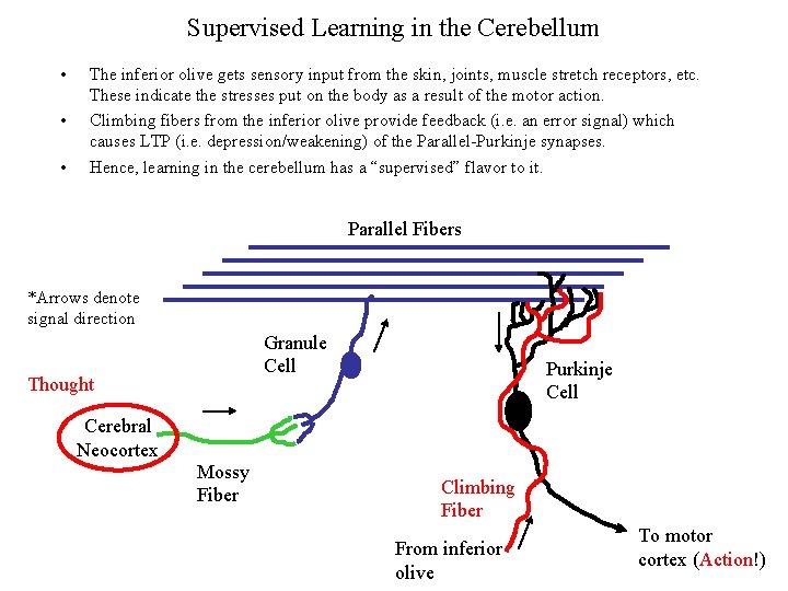
Supervised Learning in the Cerebellum • • • The inferior olive gets sensory input from the skin, joints, muscle stretch receptors, etc. These indicate the stresses put on the body as a result of the motor action. Climbing fibers from the inferior olive provide feedback (i. e. an error signal) which causes LTP (i. e. depression/weakening) of the Parallel-Purkinje synapses. Hence, learning in the cerebellum has a “supervised” flavor to it. Parallel Fibers *Arrows denote signal direction Granule Cell Thought Cerebral Neocortex Mossy Fiber Purkinje Cell Climbing Fiber From inferior olive To motor cortex (Action!)

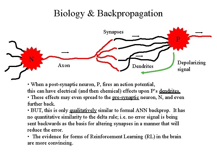
Biology & Backpropagation Synapses P N Axon Dendrites Depolarizing signal • When a post-synaptic neuron, P, fires an action potential, this can have electrical (and then chemical) effects upon P’s dendrites. • These effects may even spread to the pre-synaptic neuron, N, and even further back. • BUT, this is only qualitatively similar to formal ANN backprop. It has no quantitative similarity to the delta rule; i. e. no error signal is being sent backwards as the basis for altering synapses in a manner that will reduce the error. • The evidence forms of Reinforcement Learning (RL) in the brain are more convincing.

Backpropagation in Brain Research • Feedforward ANNs trained using backprop are useful in neurophysiology. • Given: Pairs (Sensory Inputs, Behavioral Actions) {e. g. from psychological experiments} • Backprop produces: – A general mapping/function that both • covers the I/O pairs and • can be used to PREDICT the behavioral effects of untested inputs. – A neural model of how the mapping might be wired in the brain. • The model tells neurobiologists WHAT to look for and WHERE. • So even though the means of producing the proper (trained) network is not biological, the RESULT can be very biological and useful. • The brain has so many neurons and so many connections that biologists need LOTS of help to narrow the search, both in terms of: – the structures of neural circuits in a region – The functions embodied in those circuits. • Backprop finds error minima; evolution may have also done so!

Backprop Brain Applications • Vestibular-Occular Response (VOR) : Discovering synaptic strengths in the circuitry that integrates signals from the ears (vestibular - balance and head velocity) and eyes (occular - visual images) so that we can keep our eyes focused on an object when it and/or we are moving. • LEECHNET: Tuning (hundreds of) weight parameters in the neural circuitry that governs the bending of leech body segments in response to touch stimuli. • Stereo Vision: Tuning large networks for integrating images from the right and left eye so as to detect object depth.

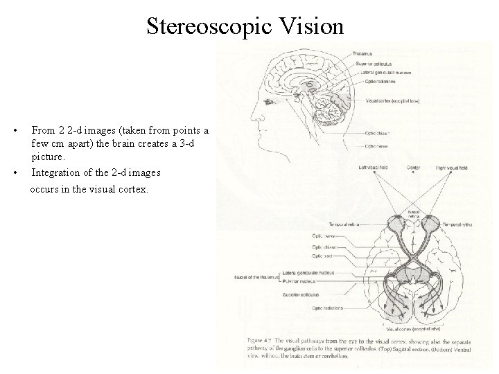
Stereoscopic Vision • • From 2 2 -d images (taken from points a few cm apart) the brain creates a 3 -d picture. Integration of the 2 -d images occurs in the visual cortex.

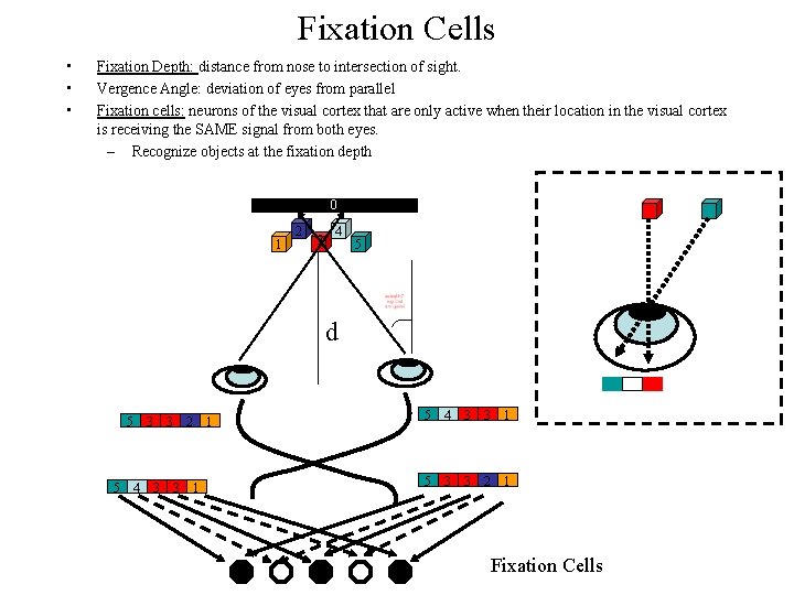
Fixation Cells • • • Fixation Depth: distance from nose to intersection of sight. Vergence Angle: deviation of eyes from parallel Fixation cells: neurons of the visual cortex that are only active when their location in the visual cortex is receiving the SAME signal from both eyes. – Recognize objects at the fixation depth 0 1 2 3 4 5 d 5 3 3 5 4 3 3 2 1 1 5 4 3 3 1 5 3 3 1 2 Fixation Cells

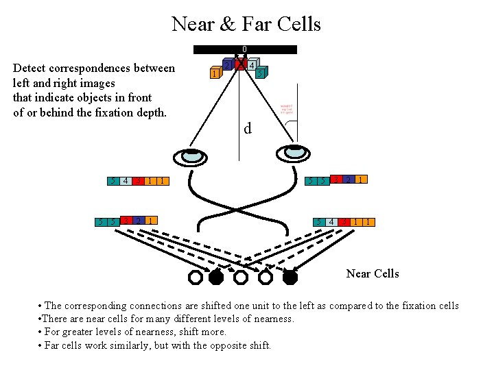
Near & Far Cells 0 Detect correspondences between left and right images that indicate objects in front of or behind the fixation depth. 5 5 4 3 1 3 2 1 5 1 1 2 3 4 5 d 5 3 5 5 4 2 3 1 1 1 Near Cells • The corresponding connections are shifted one unit to the left as compared to the fixation cells • There are near cells for many different levels of nearness. • For greater levels of nearness, shift more. • Far cells work similarly, but with the opposite shift.

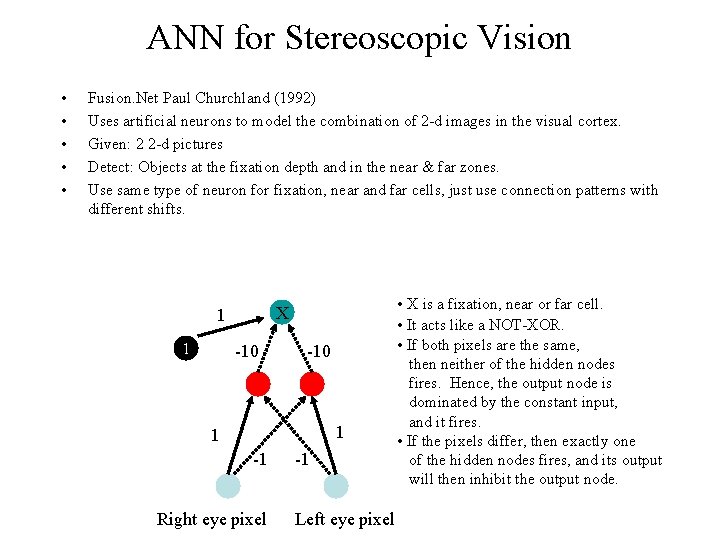
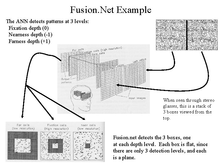
ANN for Stereoscopic Vision • • • Fusion. Net Paul Churchland (1992) Uses artificial neurons to model the combination of 2 -d images in the visual cortex. Given: 2 2 -d pictures Detect: Objects at the fixation depth and in the near & far zones. Use same type of neuron for fixation, near and far cells, just use connection patterns with different shifts. X 1 1 -10 1 1 -1 Right eye pixel -1 Left eye pixel • X is a fixation, near or far cell. • It acts like a NOT-XOR. • If both pixels are the same, then neither of the hidden nodes fires. Hence, the output node is dominated by the constant input, and it fires. • If the pixels differ, then exactly one of the hidden nodes fires, and its output will then inhibit the output node.

Fusion. Net Example The ANN detects patterns at 3 levels: Fixation depth (0) Nearness depth (-1) Farness depth (+1) When seen through stereo glasses, this is a stack of 3 boxes viewed from the top. Fusion. net detects the 3 boxes, one at each depth level. Each box is flat, since there are only 3 detection levels, and each is a plane.

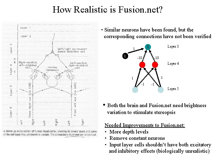
How Realistic is Fusion. net? • Similar neurons have been found, but the corresponding connections have not been verified 1 Layer 3 X 1 -10 Layer 4 1 1 -1 -1 Layer 5 • Both the brain and Fusion. net need brightness variation to stimulate stereopsis Needed Improvements to Fusion. net: • More depth levels • Remove constant neurons • Input layer cells shouldn’t have both excitatory and inhibitory effects (biologically unrealistic)