Supervised Feature Selection Unsupervised Dimensionality Reduction Feature Subset
Supervised Feature Selection & Unsupervised Dimensionality Reduction
Feature Subset Selection • Supervised: class labels are given • Select a subset of the problem features • Why? – Redundant features • much or all of the information contained in one or more other features • Example: purchase price of a product and the amount of sales tax – Irrelevant features • contain no information that is useful for the data mining task at hand • Example: students' ID is often irrelevant to the task of predicting students' GPA • Data mining may become easier • The selected features may convey important information (e. g. gene selection)
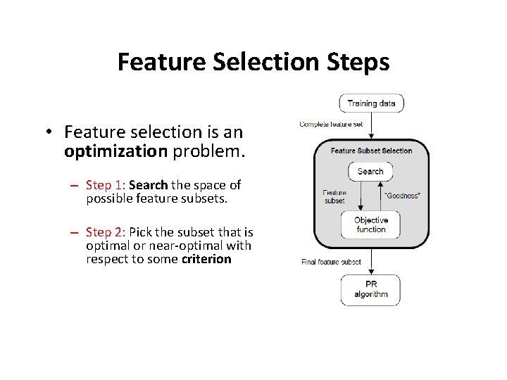
Feature Selection Steps • Feature selection is an optimization problem. – Step 1: Search the space of possible feature subsets. – Step 2: Pick the subset that is optimal or near-optimal with respect to some criterion

Feature Selection Steps (cont’d) Search strategies – Exhaustive – Heuristic Evaluation Criterion - Filter methods - Wrapper methods Embedded methods
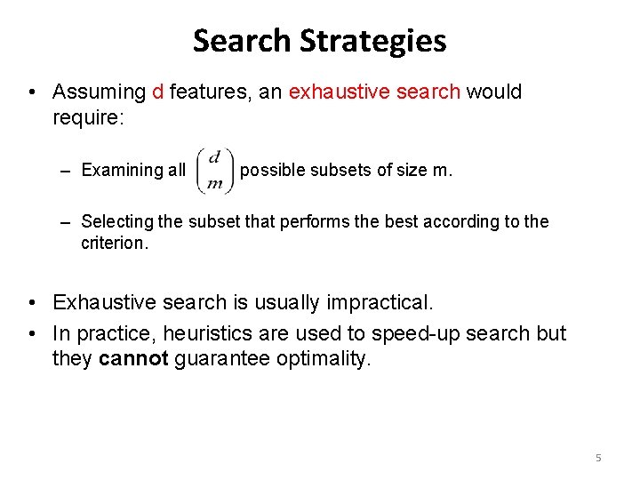
Search Strategies • Assuming d features, an exhaustive search would require: – Examining all possible subsets of size m. – Selecting the subset that performs the best according to the criterion. • Exhaustive search is usually impractical. • In practice, heuristics are used to speed-up search but they cannot guarantee optimality. 5
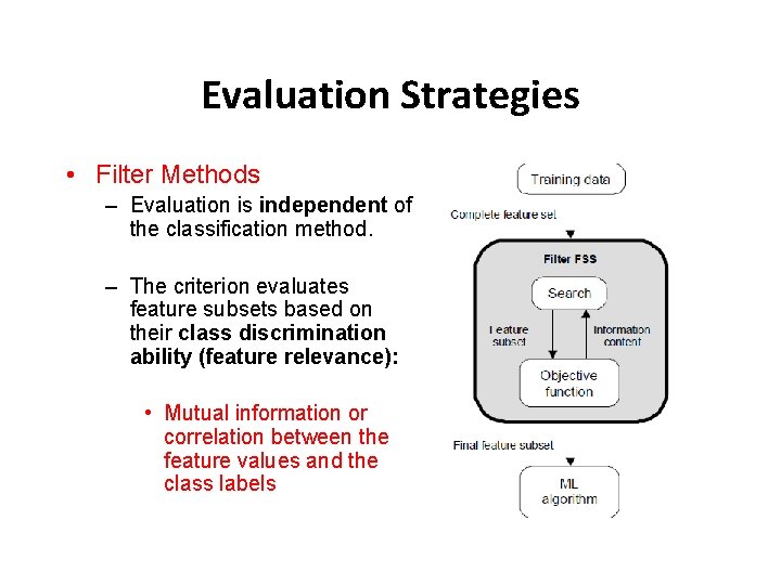
Evaluation Strategies • Filter Methods – Evaluation is independent of the classification method. – The criterion evaluates feature subsets based on their class discrimination ability (feature relevance): • Mutual information or correlation between the feature values and the class labels
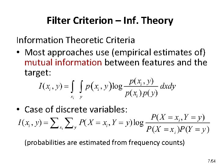
Filter Criterion – Inf. Theory Information Theoretic Criteria • Most approaches use (empirical estimates of) mutual information between features and the target: • Case of discrete variables: (probabilities are estimated from frequency counts) 7/54
Filter Criterion - SVC Single Variable Classifiers • Idea: Select variables according to their individual predictive power • criterion: Performance of a classifier built with 1 variable • e. g. the value of the variable itself (decision stump) (set treshold on the value of the variable) • predictive power is usually measured in terms of error rate (or criteria using presicion, recall, F 1)
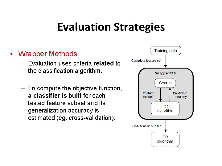
Evaluation Strategies • Wrapper Methods – Evaluation uses criteria related to the classification algorithm. – To compute the objective function, a classifier is built for each tested feature subset and its generalization accuracy is estimated (eg. cross-validation).
Feature Ranking • Evaluate all d features individually using the criterion • Select the top m features from this list. • Disadvantage – Correlation among features is not considered
Sequential forward selection (SFS) (heuristic search) • First, the best single feature is selected (i. e. , using some criterion). • Then, pairs of features are formed using one of the remaining features and this best feature, and the best pair is selected. • Next, triplets of features are formed using one of the remaining features and these two best features, and the best triplet is selected. • This procedure continues until a predefined number of features are selected. • Wrapper methods (e. g. decision trees, linear classifiers) or Filter methods (e. g. m. RMR) could be used 11
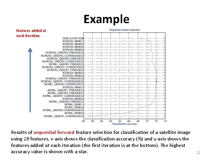
Example features added at each iteration Results of sequential forward feature selection for classification of a satellite image using 28 features. x-axis shows the classification accuracy (%) and y-axis shows the features added at each iteration (the first iteration is at the bottom). The highest accuracy value is shown with a star. 12
Sequential backward selection (SBS) (heuristic search) • First, the criterion is computed for all n features. • Then, each feature is deleted one at a time, the criterion function is computed for all subsets with n-1 features, and the worst feature is discarded. • Next, each feature among the remaining n-1 is deleted one at a time, and the worst feature is discarded to form a subset with n-2 features. • This procedure continues until a predefined number of features are left. • Wrapper or filter methods could be used. 13
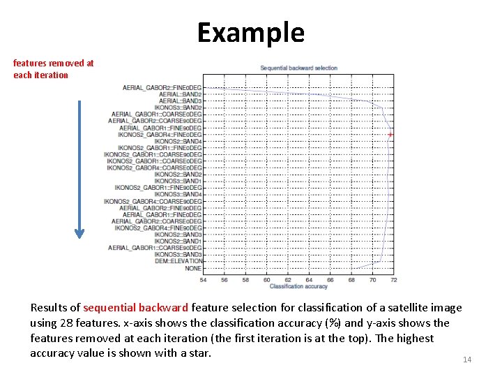
Example features removed at each iteration Results of sequential backward feature selection for classification of a satellite image using 28 features. x-axis shows the classification accuracy (%) and y-axis shows the features removed at each iteration (the first iteration is at the top). The highest accuracy value is shown with a star. 14
Limitations of SFS and SBS • The main limitation of SFS is that it is unable to remove features that become redundant after the addition of other features. • The main limitation of SBS is its inability to reevaluate the usefulness of a feature after it has been discarded.
Embedded Methods • • Tailored to a specific classifier RFE-SVM: – RFE: Recursive Feature Elimination – Iteratively train a linear SVM and remove features with the smallest weights at each iteration – Has been successfully used for gene selection in bioinformatics • Decision Trees or Random Forest: evaluate every feature by computing average reduction in impurity for the tree nodes containing this feature • Random Forest: determine the importance of a feature by measuring how the out-of-bag error of the classifier will be increased, if the values of this feature in the out-of-bag samples are randomly permuted • Relief (based on k-NN): the weight of any given feature decreases if its value differs in nearby instances of the same class more than it differs in nearby instances of the other class (and increases in the opposite case).
Unsupervised Dimensionality Reduction • Feature Extraction: new features are created by combining the original features • The new features are usually fewer than the original • No class labels available (unsupervised) • Purpose: – Avoid curse of dimensionality – Reduce amount of time and memory required by data mining algorithms – Allow data to be more easily visualized – May help to eliminate irrelevant features or reduce noise • Techniques – Principal Component Analysis (optimal linear approach) – Non-linear approaches
PCA: The Principal Components • Vectors originating from the center of the dataset (data centering: use (x-m) instead of x, m=mean(X)) • Principal component #1 points in the direction of the largest variance. • Each subsequent principal component… – is orthogonal to the previous ones, and – points in the directions of the largest variance of the residual subspace
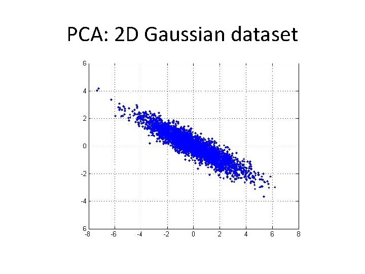
PCA: 2 D Gaussian dataset
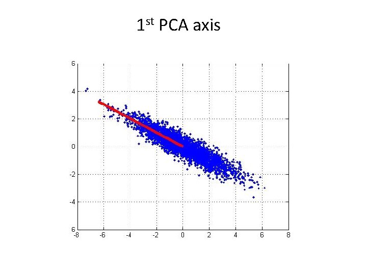
1 st PCA axis
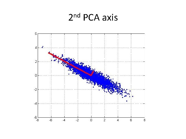
2 nd PCA axis
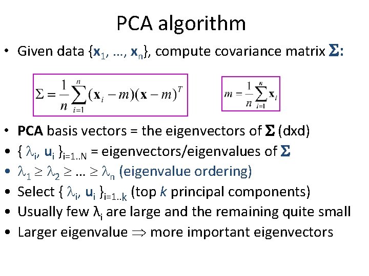
PCA algorithm • Given data {x 1, …, xn}, compute covariance matrix : • • • PCA basis vectors = the eigenvectors of (dxd) { i, ui }i=1. . N = eigenvectors/eigenvalues of 1 2 … n (eigenvalue ordering) Select { i, ui }i=1. . k (top k principal components) Usually few λi are large and the remaining quite small Larger eigenvalue more important eigenvectors
![PCA algorithm • • W=[u 1 u 2 … uk ]T (kxd projection matrix) PCA algorithm • • W=[u 1 u 2 … uk ]T (kxd projection matrix)](http://slidetodoc.com/presentation_image_h2/99141c2f0c41ce9d8512bb868318bb9e/image-23.jpg)
PCA algorithm • • W=[u 1 u 2 … uk ]T (kxd projection matrix) Z=X*WT (nxk data projections) Xrec=Z*W (nxd reconstructions of X from Z) PCA is optimal Linear Projection: minimizes the reconstruction error:
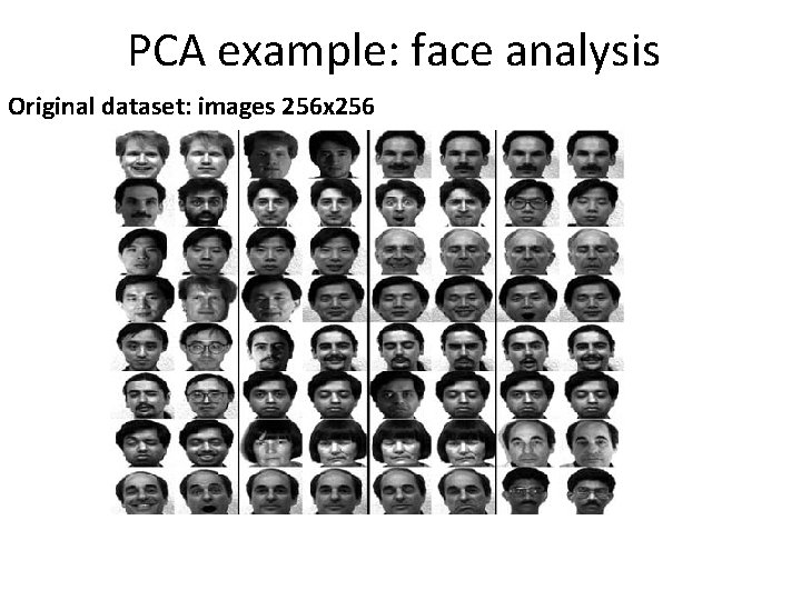
PCA example: face analysis Original dataset: images 256 x 256
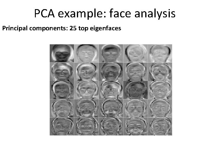
PCA example: face analysis Principal components: 25 top eigenfaces
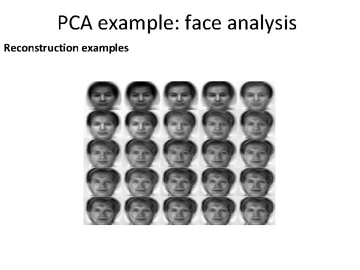
PCA example: face analysis Reconstruction examples
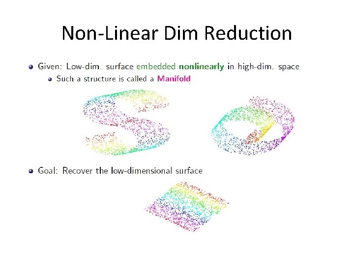
Non-Linear Dim Reduction • rerwerwer
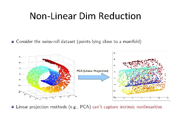
Non-Linear Dim Reduction
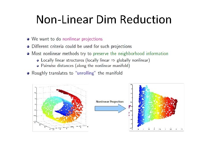
Non-Linear Dim Reduction
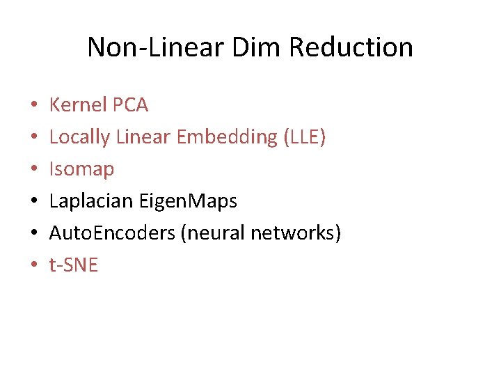
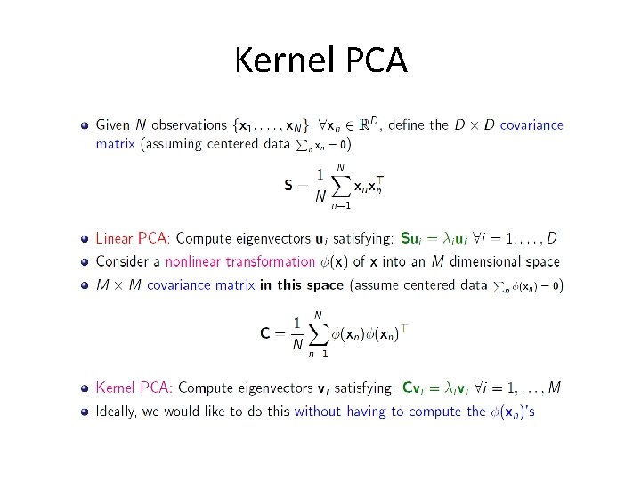
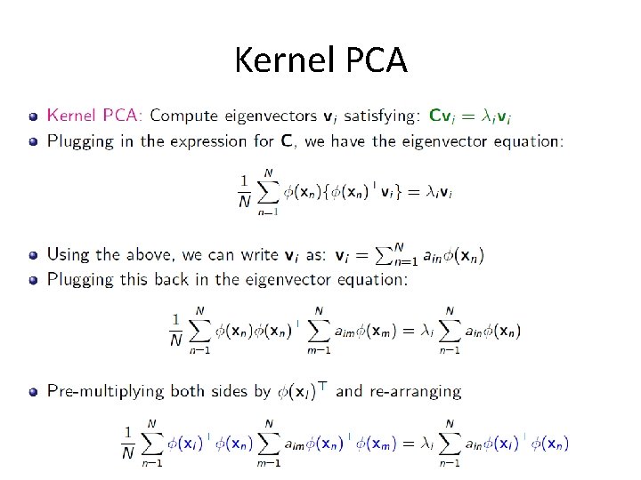
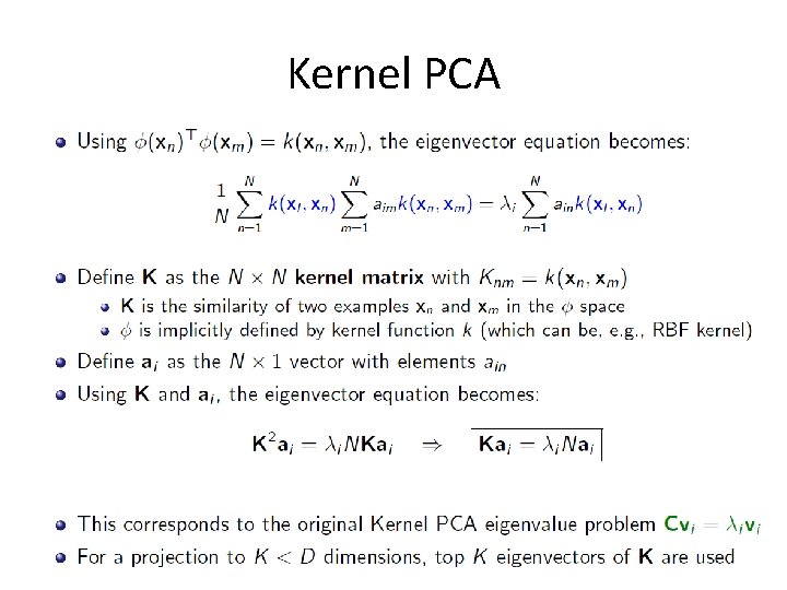
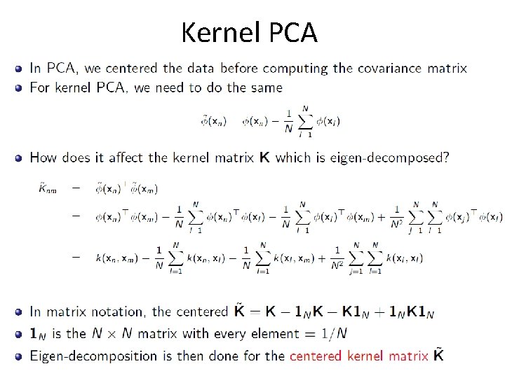
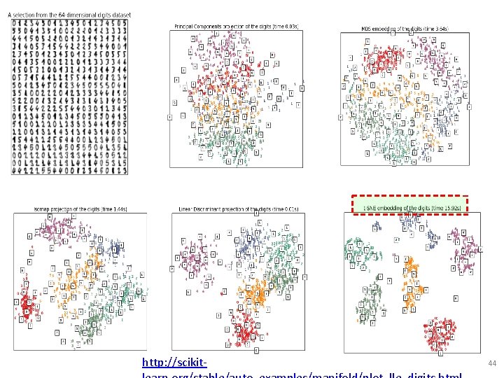
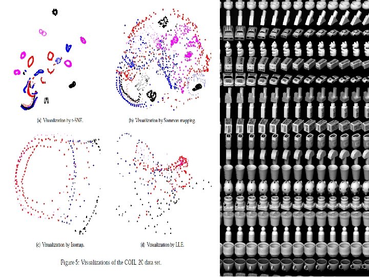
Non-Linear Dim Reduction • • • Kernel PCA Locally Linear Embedding (LLE) Isomap Laplacian Eigen. Maps Auto. Encoders (neural networks) t-SNE
Kernel PCA
Kernel PCA
Kernel PCA
Kernel PCA
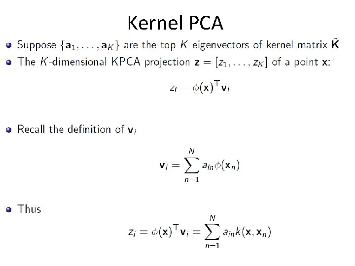
Kernel PCA
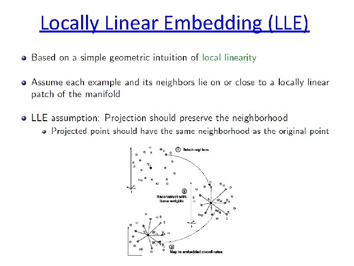
Locally Linear Embedding (LLE)
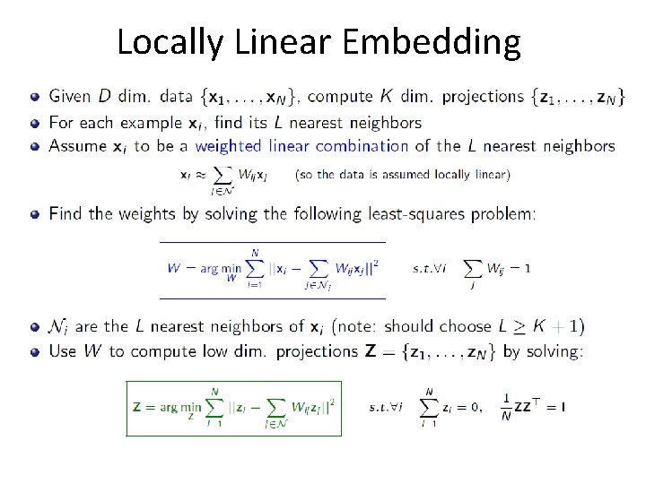
Locally Linear Embedding
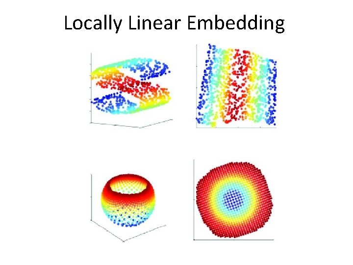
Locally Linear Embedding
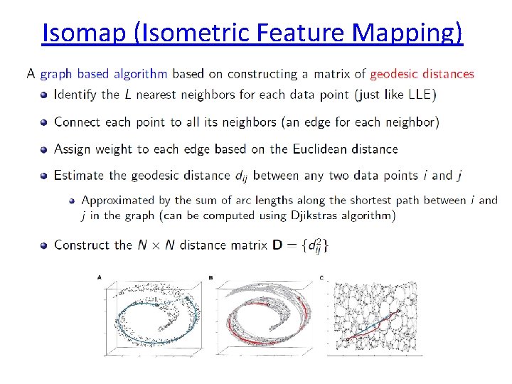
Isomap (Isometric Feature Mapping)
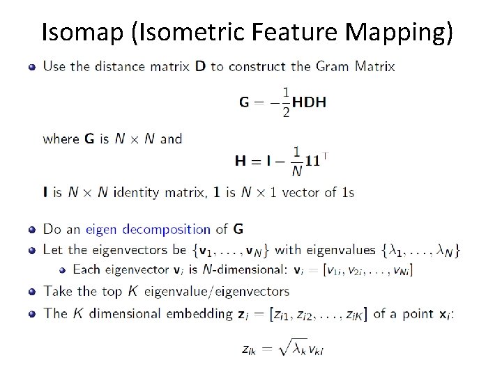
Isomap (Isometric Feature Mapping)
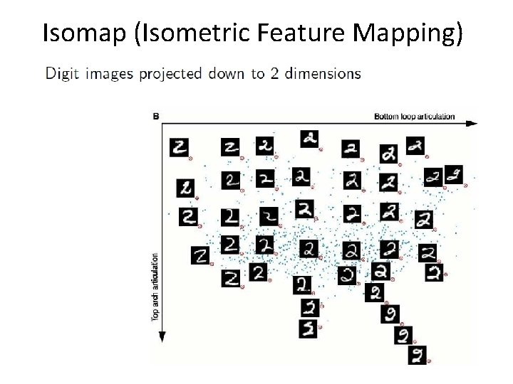
Isomap (Isometric Feature Mapping)
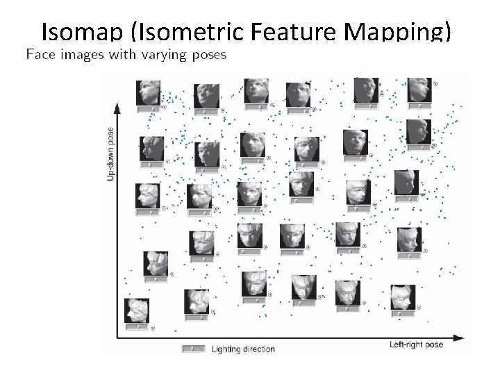
Isomap (Isometric Feature Mapping)

Visualizing Data using t-SNE Laurens van der Maaten, and Geoffrey Hinton Tilburg University. The Netherlands University of Toronto. Canada Journal of Machine Learning Research (2008) slides from→ http: //kawahara. ca/visualizing-data-using-t-sne-slides/ 43
http: //scikit- 44
45
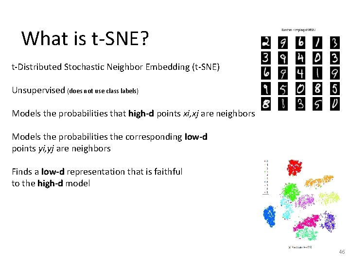
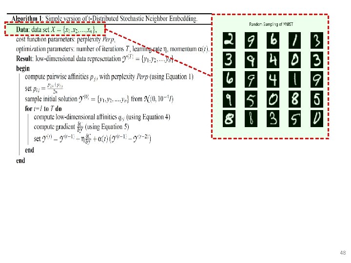
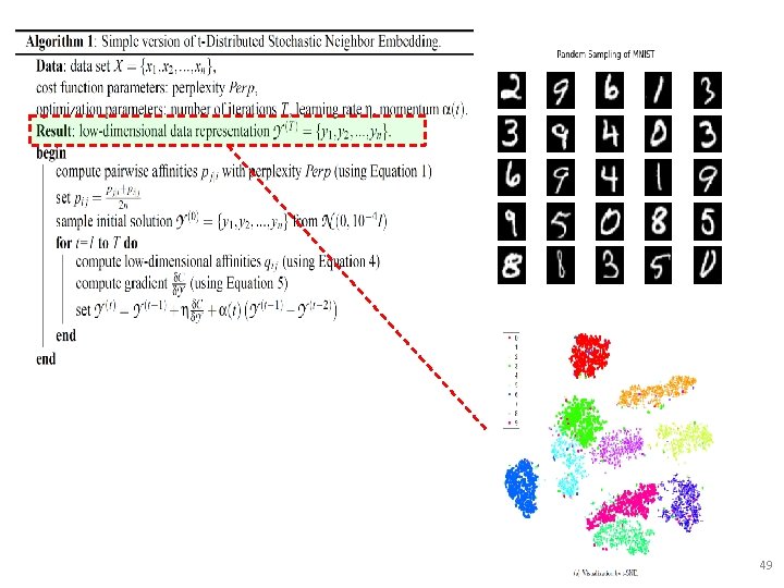
What is t-SNE? t-Distributed Stochastic Neighbor Embedding (t-SNE) Unsupervised (does not use class labels) Models the probabilities that high-d points xi, xj are neighbors Models the probabilities the corresponding low-d points yi, yj are neighbors Finds a low-d representation that is faithful to the high-d model 46
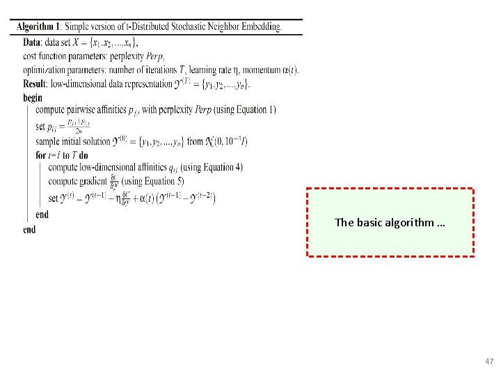
The basic algorithm … 47
48
49
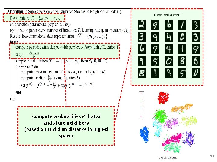
Compute probabilities P that xi and xj are neighbors (based on Euclidian distance in high-d space) 50
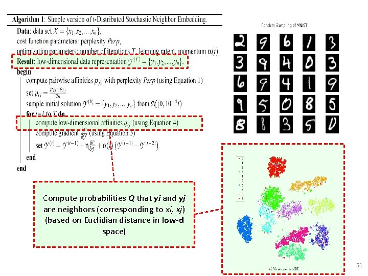
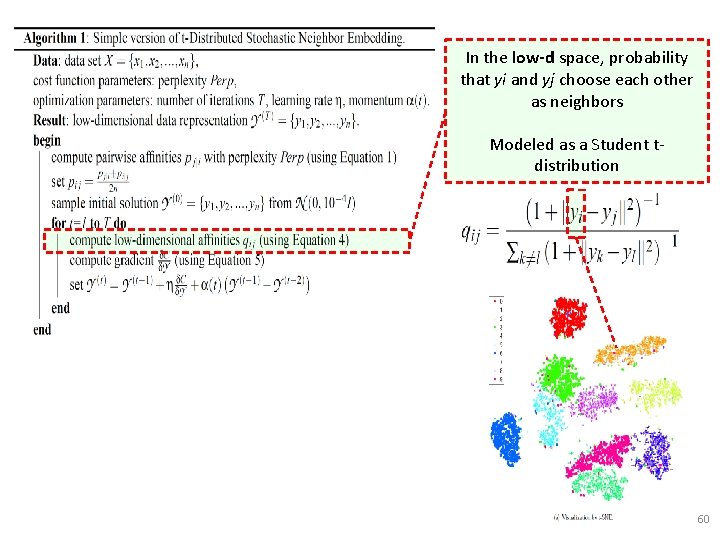
Compute probabilities Q that yi and yj are neighbors (corresponding to xi, xj) (based on Euclidian distance in low-d space) 51
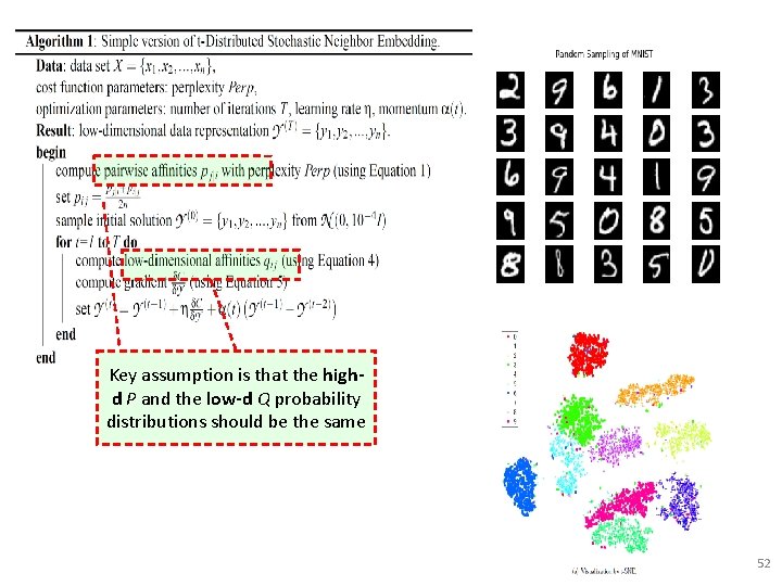
Key assumption is that the highd P and the low-d Q probability distributions should be the same 52
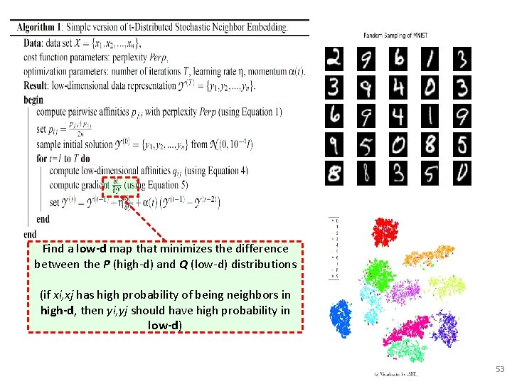
Find a low-d map that minimizes the difference between the P (high-d) and Q (low-d) distributions (if xi, xj has high probability of being neighbors in high-d, then yi, yj should have high probability in low-d) 53
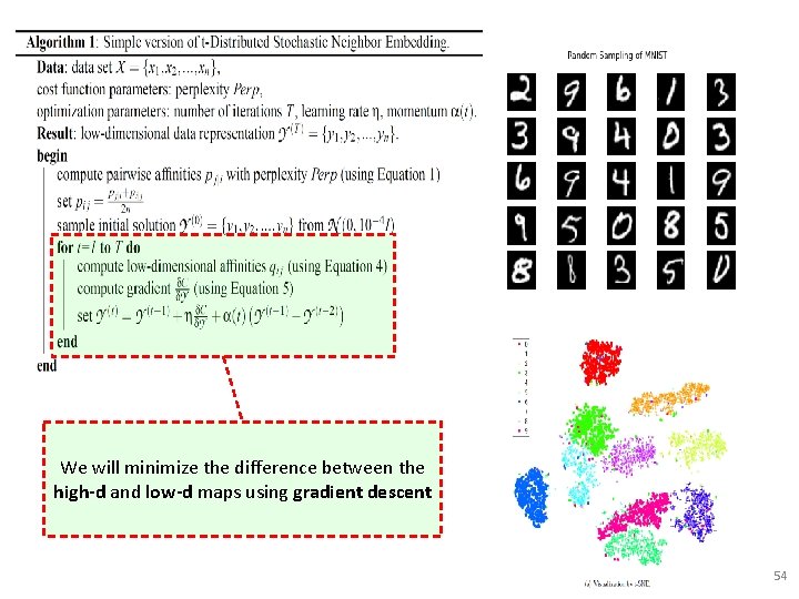
We will minimize the difference between the high-d and low-d maps using gradient descent 54
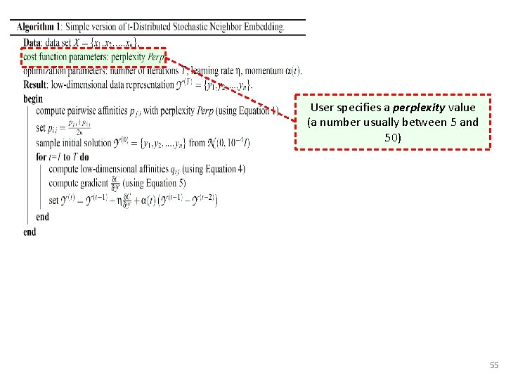
User specifies a perplexity value (a number usually between 5 and 50) 55
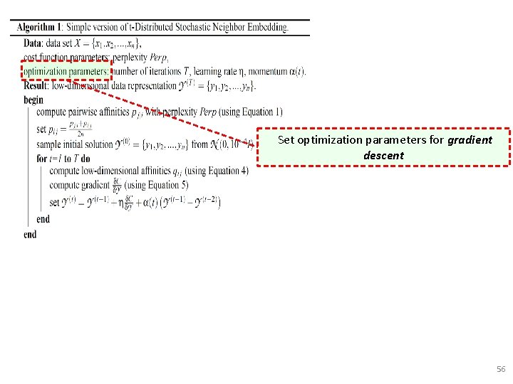
Set optimization parameters for gradient descent 56
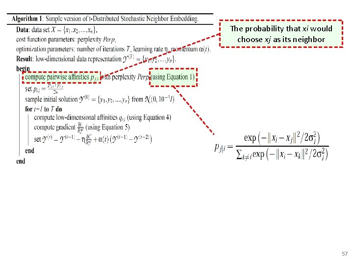
The probability that xi would choose xj as its neighbor 57
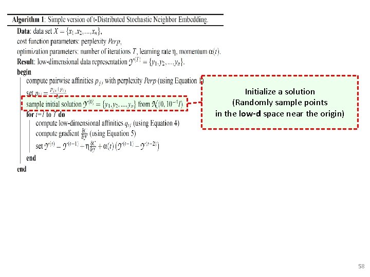
Initialize a solution (Randomly sample points in the low-d space near the origin) 58
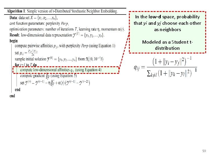
In the low-d space, probability that yi and yj choose each other as neighbors Modeled as a Student tdistribution 59
In the low-d space, probability that yi and yj choose each other as neighbors Modeled as a Student tdistribution 60
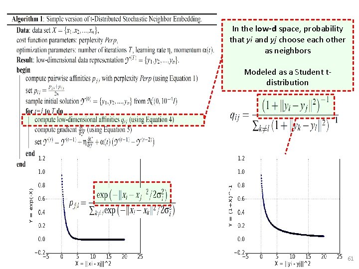
In the low-d space, probability that yi and yj choose each other as neighbors Modeled as a Student tdistribution 61
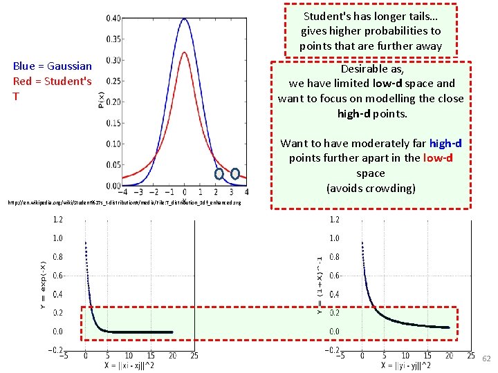
Blue = Gaussian Red = Student's T Student's has longer tails… gives higher probabilities to In that the low-d space, away probability points are further that yi and yj choose each other Desirable as, as neighbors we have limited low-d space and want to focus on modelling the close Modeled as a Student thigh-ddistribution points. Want to have moderately far high-d points further apart in the low-d space (avoids crowding) http: //en. wikipedia. org/wiki/Student%27 s_t-distribution#/media/File: T_distribution_1 df_enhanced. svg 62
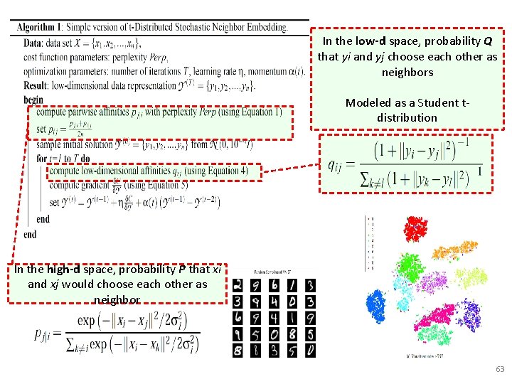
In the low-d space, probability Q that yi and yj choose each other as neighbors Modeled as a Student tdistribution In the high-d space, probability P that xi and xj would choose each other as neighbor 63
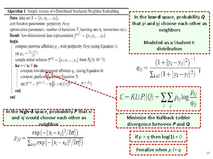
In the low-d space, probability Q that yi and yj choose each other as neighbors Modeled as a Student tdistribution In the high-d space, probability P that xi and xj would choose each other as neighbor Minimize the Kullback-Leibler divergence between P and Q if p = q then log(1) = 0 Penalize when p != q 64
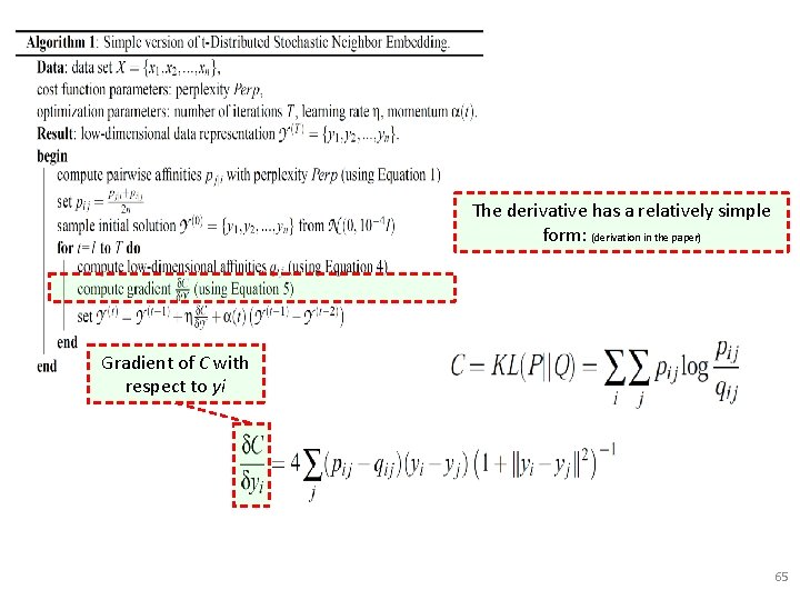
The derivative has a relatively simple form: (derivation in the paper) Gradient of C with respect to yi 65
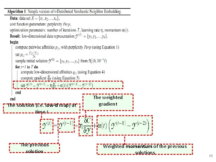
The solution (i. e. low-d map) at time t The previous solution The weighted gradient Weighted momentum of the previous solutions 66
- Slides: 66