Superconducting Flux Qubit as a Macroscopic Artificial Atom

Superconducting Flux Qubit as a Macroscopic Artificial Atom Hideaki Takayanagi NTT Basic Research Laboratories, NTT Corporation, Japan NTT物性科学基礎研究所 髙柳英明 Outline 1. 2. 3. 4. 5. 6. Quantum Information Research at NTT Fux Qubit Single-Shot Measurement Multi-Photon Absorption Rabi Oscillation Conclusions

QIT Project in NTT Basic Research Laboratories Head: H. Takayanagi About 20 researchers participate to the project which consists of five sub-projects. Four qubit-research projects and a quantum cryptography one.

Four Kinds of Qubit SQUID Single-shot measurement Multi-photon absorption Rabi oscillation Solid-State Qubits Coupled QDs (artificial molecule) Rabi oscillation Exciton in QDs Quantum gate operation cooled atom Atom Chip

Quantum cryptography with a single photon Testing Alice Helium Cryostat Titanium-Sapphire Laser Counter Space filter Bob Photon 0 Half-wavelength waveguide 電気光学 変調器 Quantumlens Lens dot Pin-hole Single-mode fiber Beam Splitter Mirror Grating Attenuator Detector 3 50%-50% ¼ wavelength Beam Splitter Detector 4 Beam Splitter Detector 1 Lens Detector 2 時間間隔 解析器 Generator Amp 時間間隔 解析器 Nature, 420 (2002) 762

Josephson persistent current Qubit J. E. Mooij et al. , Science 285, 1036 (1999). EJ , g 3 B Phase difference qubit = f 0 gq = g 1 + g 2 + g 3 = 2 p f f = qubit / 0 E J , g 2 E J , g 1 Josephson Energy : U = EJ ( 2 + a jp jm - cosg 1 - cosg 2 - a f = qubit / 0 = 0. 5 g 2 jp = j g 1 1 2 1 m= 2 ( g 1 + g 2 ) ( g 1 - g 2 ) cos ( 2 p f - g 1 - g 2 ) ) U =0. 6 =0. 8 =1. 0 jp jm

Schematic qubit energy spectrum 15 -100 0. 4 0. 5 qubit/ 0 0. 6 10 5 D 0 Energy (GHz) 100 -5 -10 0. 49 0. 50 qubit / 0 0. 51

Three-Josephson-junction Loop: Description 0< <1. 0 E J 1 C EJ ; C 3 ext= f 0 • Josephson Energy (1 junction): 2 E J C • Coupling energy (1 junction): EC = e 2/ 2 C • Flux quantization: Josephson Energy: J. E. Mooij､et al (1999)

Three-Josephson-junction Loop: Energy Diagram f=0. 5 U 2 minima in each unit cell. Top View

Three-Josephson-junction Loop: Dependence of the Potential f=0. 5 U U U =0. 6 =0. 8 If increases, the barrier height : • increases between the two minima of one unit cell • decreases between the minima of adjacent cells =1. 0

Three-Josephson-junction Loop: Flux Dependence of the States Classical states = persistent currents of opposite sign. Degenerated at f = 0. 5 Quantum tunnelling “anti-crossing” E 0 (1) Level splitting E <Iq>/Ip Symmetric and antisymmetric superposition of the macroscopic persistent currents / 0 Classical states Quantum ground state |0> Quantum first excited state |1>

Sample Fabrication • • • Qubit and a detector dc-SQUID NTT Atsugi e-beam lithography Shadow evaporation Lift-off Josephson junctions Al / Al 2 O 3 / Al Junction area SQUID : 0. 1 x 0. 08 m 2 Qubit : 0. 1 x L m 2, ( = 0. 8 ) L = 2 ~ 0. 2 Loop size SQUID ~ 7 x 7 m 2 Qubit ~ 5 x 5 m 2 Mutual inductance M ~ 7 p. H

e-beam lithography suspended-bridge & shadow evapolation

DC measurement Sample and Cavity To mixing chamber Thermometer Ibias line Microwave line Vm line NTT Atsugi Samples A loop Cavity

1 R. T. 2 3 DC measurement RF line 5 4 10 n. F HP 20 d. B 4. 2 K Flexible coaxial cable HP 10 d. B connectors 2. 4 mm connectors Through capacitor 1. 2 K attenuator 0. 8 K resistance 0. 4 K 10 m. K Heat anchor for outer shield Twisted Constantan wire 100 200 Sample box 200 • No on-chip capacitor and resistor • No on-chip control line • Change twisted wires to thin coaxial cables to introduce dc-pulse Loop antenna ~ 1 mm above the sample

DC measurement Readout through a dc-SQUID I b Sweep Ib ( 140 Hz ) Tilt SQUID potential Vm qubit Record each switching when Vm = Vth~ 30 V as a function of Isw Ib ~ 100 n. A Isw 4~6 n. A Isw Isw 0 t 70 ~ 100 μsec Vm Vth(~30μV) 0 ~ 7 ms t

DC measurement Readout with a dc-SQUID Current is swept I(V) curve Magnetic field is swept Isw( / 0) curve

DC measurement Qubit step in the SQUID Isw Qubit switches its current sign Flux in SQUID changes through M SQUID Isw changes Φ M Qubit dc-SQUID qubit / 0 Step on the Isw( / 0)

Parameter dependence of the qubit step ( D, Ej, Ec ) SQUID I Qubit Lqubit LSQUID Josephson junctions : Al / Al 2 O 3 / Al Junction area : SQUID 0. 2 x 0. 2 m 2 qubit 0. 2 x L m 2, L=0. 3, 0. 5, 1. 0 Loop size : Lqubit = 5. 1, 9. 7, 19. 0 ( m) LSQUID = 6. 3, 10. 9, 20. 2

Two energy scale Ec, EJ Pair tunneling superconductor Tunnel barrier energy Number of tunneled pair n H = Ec - EJ cos g - Iex g energy -p p Phase difference [n, g]=i Josephson energy : EJ charging energy : Ec =(2 ne)2/(2 CJ ) k. BT << EJ << Ec < D →　charge qubit 　　　　　 k. BT << Ec << EJ < D →　phase、flux qubit

QB# 6 Junction area = 0. 2 m 2 Loop size : Lqubit = 9. 7 m LSQUID = 10. 9 m ( D ~ 2 MHz << k. BT ) qubit / 0 QB# 3 Junction area = 0. 2 m 2 Loop size : Lqubit = 5. 1 m LSQUID = 6. 3 m qubit / 0 QB# 5 Junction area = 0. 1 m 2 Loop size : Lqubit = 9. 7 m LSQUID = 10. 9 m ( D ~ 0. 4 GHz ~ k. BT ) qubit / 0 QB# 8 Junction area = 0. 1 m 2 Loop size : Lqubit = 19. 0 m LSQUID = 20. 2 m qubit / 0 k. BT~25 m. K QB# 4 Junction area = 0. 06 m 2 Loop size : Lqubit = 9. 7 m LSQUID = 10. 9 m ( D ~ 2 GHz > k. BT ) qubit / 0 QB# 7 Junction area = 0. 06 m 2 Loop size : Lqubit = 19. 0 m LSQUID = 20. 2 m qubit / 0 Qubit energy splitting D

Calculated qubit energy level D=0. 4 GHz D=2 MHz Ej=544 GHz Ec=1. 6 GHz Ej=280 GHz Ec=3. 2 GHz Ej=130 GHz Ec=5. 4 GHz

Optimal operation point for SQUID Qubit signals appear at half-integer Sensitivity of dc-SQUID depends on magnetic fields We can achieve excellent resolution at f = 1. 5 ↓ ↑

Spectroscopy EJ = 312 GHz, EC = 3. 8, = 0. 7 D = 2. 6 GHz after averaging 0. 001 0 M 2. 4 GHz w/o averaging

DC measurement Qubit signals at different SQUID modulation S/N depends on SQUID Isw design qubit and SQUID to be crossed at small Isw | > | > T = 25 m. K

E 0 (1) Level splitting E <Iq>/Ip f= / 0 Classical states Quantum ground state |0> Quantum first excited state |1>

Boltzman Distribution E 0 (1) Level splitting E <Iq>/Ip / 0 Classical states Quantum ground state |0> Quantum first excited state |1>

Schematic qubit energy spectrum 15 -100 0. 4 0. 5 qubit/ 0 0. 6 10 5 D 0 Energy (GHz) 100 -5 -10 0. 49 0. 50 qubit / 0 0. 51

Spectroscopy DC measurement Pulse measurement D excited state ground state

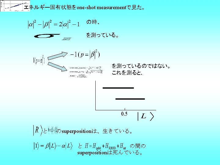
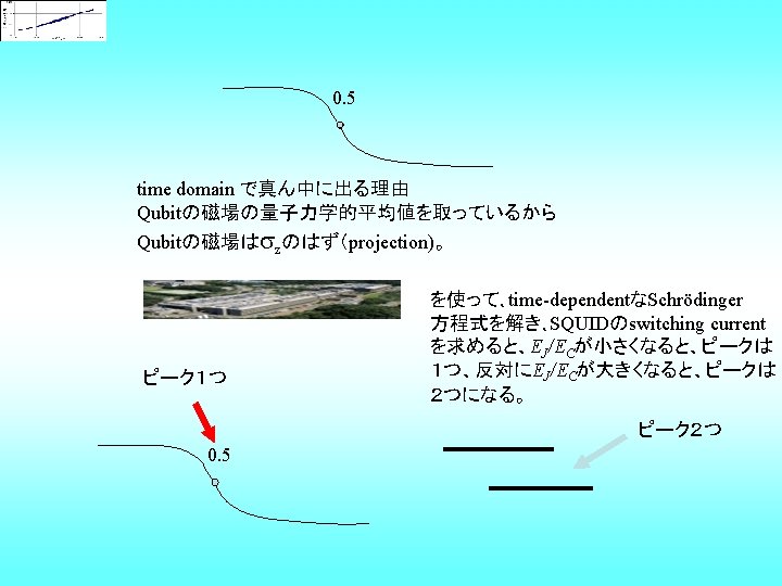
Readout without averaging Single shot measurement into { l 0>, l 1> } bases The <Iq> step shape does not change. Only the population changes. qubit / 0 DC measurement

DC measurement Close-up of Isw, T=25 m. K Histogram is well separated ! counts f qubit / 0 f = 1. 50102 counts 0. 001 0 M 2. 4 GHz

Readout after averaging DC measurement Expected Current ( canonical ensemble average ) qubit / 0

Pulse measurement Experimental setup 1 2 3 4 5 RF line SLP-1. 9 R. T. 4. 2 K RFin : ２ attenuators Flexible coaxial cable RFout : terminator 1. 2 K + attenuator 0. 8 K DC : LP filter + Meander filter I- I+ V+V- HP 10 d. B 0. 4 K 29 m. K Thin coaxial cable f 0. 33 mm Meander filters Weinschell 10 d. B Sample cavity RF in Sample cavity Terminator 50 RF in On-chip strip line

Multi-photon transition between superposition of macroscopic quantum states ｰ ( ) /√ 2　 1 st excited state ＋ ( ) /√ 2　 ground state 3 2 1 1 2 3

Multi-photon transition Multi-photon spectroscopy SQUID readout 2 RF : 3. 8 GHz -10 d. Bm d I SW (n. A) 1 0 3 2 １ D=0. 86 GHz 2 -1 1 -photon １ -2 1. 496 1. 498 1. 500 qubit / 0 2 1. 502 RF : 3. 8 GHz 0 d. Bm d I SW (n. A) 1 0 1. 504 １ 3 2 -1 -2 1. 496 2 1. 498 １ 1. 500 / 0 qubit 1. 502 1. 504 2 -photon

Multiphoton absorption at 9. 1 GHz RF Power dependence triple double single off off 0 d. Bm PRF = - 21 d. Bm 9. 6 d. Bm 13. 2 d. Bm 10 d. Bm 12 d. Bm

Multi-photon transition Peak width vs MW intensity Bloch Kinetic Equation 9100 MHz ----- (3) --------- (4)

Pulse measurement scheme repetition: 3 k. Hz ( 333 s) 180 ns ~1μs SQUID switch Ib DC pulse Non-switching time resonant microwave MW discrimination of the switching event Vout + I bias Ibias + Vout ext SQUID V th Switching events Ibias - Non-switching events Switching event

030304_1 (1, 2)FQB 2 Pulse measurement Relaxation time T 1 9. 1 GHz 1 s pulse 1 st excited sate 10 5 55 MW D 0 -5 Ground state -10 0. 49 0. 50 0. 51 qubit / 0 500 ns 3 s 1 s delay time Ib pulse height 1. 474 V, Trailing height ratio 0. 6 Probability [%] Energy (GHz) 15 50 data exp-fit 45 T 1 = 1. 6 s 40 35 30 25 0 1 2 Delay Time [ s]

Pulse measurement Quantum Oscillation : Rabi oscillations 11. 4 GHz Dephasing time ~ 30 ns 150 ns 600 s Trailing height ratio 0. 7 NTT Atsugi switching probability ( % ) Rabi frequency ( MHz ) Resonant MW pulse width MW amplitude (a. u. ) pulse width ( ns )

Summary • Spectroscopy of MQ artificial 2 -level system • Qubit readout without averaging (DC) • Multi-photon transition between superposed MQ states • Coherent quantum oscillation ( Rabi oscillation ) • T 1 ~1. 6 s, T 2 Rabi ~ 30 ns Future plan • Ramsey, Spin echo • Two qubit fabrication and operation • MQC with single shot resolution

collaborators NTT Basic Research Laboratories Hirotaka Tanaka Shiro Saito Hayato Nakano Frank Deppe Takayoshi Meno Kouich Semba Tokyo Institute of Technology Masahito Ueda Yokohama National University Yoshihiro Shimazu Tomoo Yokoyama Tokyo Science University Takuya Mouri Tatsuya Kutsuzawa