SumProduct Networks A New Deep Architecture Pedro Domingos

Sum-Product Networks: A New Deep Architecture Pedro Domingos Dept. Computer Science & Eng. University of Washington Joint work with Hoifung Poon 1

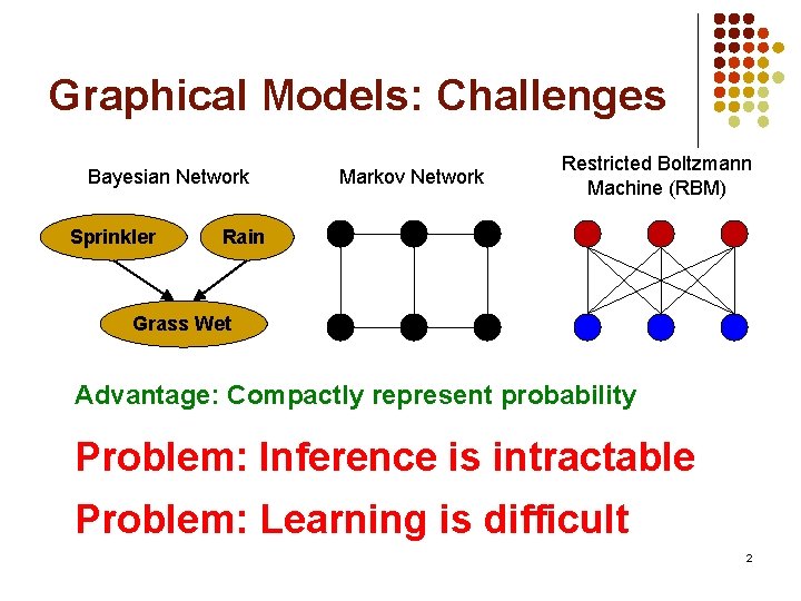
Graphical Models: Challenges Bayesian Network Sprinkler Markov Network Restricted Boltzmann Machine (RBM) Rain Grass Wet Advantage: Compactly represent probability Problem: Inference is intractable Problem: Learning is difficult 2

Deep Learning l Stack many layers E. g. : DBN [Hinton & Salakhutdinov, 2006] CDBN [Lee et al. , 2009] DBM [Salakhutdinov & Hinton, 2010] l Potentially much more powerful than shallow architectures [Bengio, 2009] l But … l Inference is even harder l Learning requires extensive effort 3

Learning: Requires approximate inference Inference: Still approximate Graphical Models

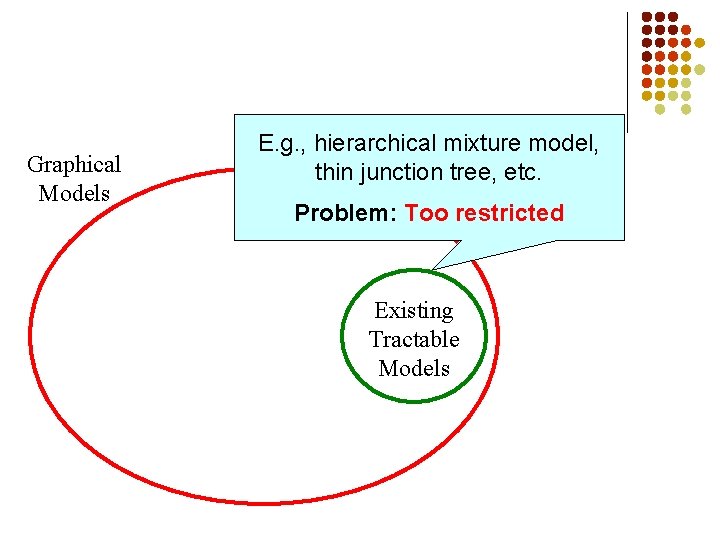
Graphical Models E. g. , hierarchical mixture model, thin junction tree, etc. Problem: Too restricted Existing Tractable Models

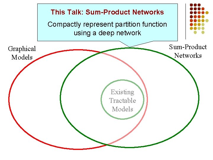
This Talk: Sum-Product Networks Compactly represent partition function using a deep network Sum-Product Networks Graphical Models Existing Tractable Models

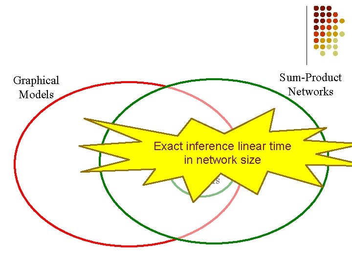
Sum-Product Networks Graphical Models Exact. Existing inference linear time in network size Tractable Models

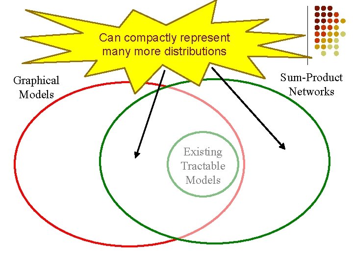
Can compactly represent many more distributions Sum-Product Networks Graphical Models Existing Tractable Models

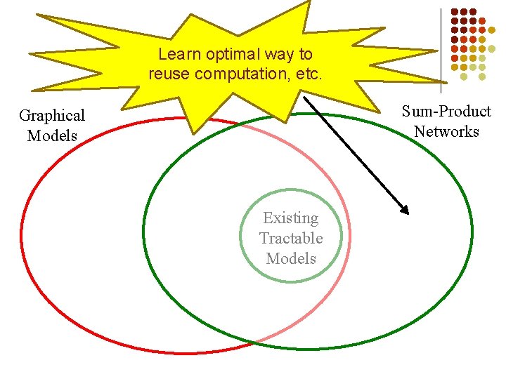
Learn optimal way to reuse computation, etc. Sum-Product Networks Graphical Models Existing Tractable Models

Outline l l Sum-product networks (SPNs) Learning SPNs Experimental results Conclusion 10

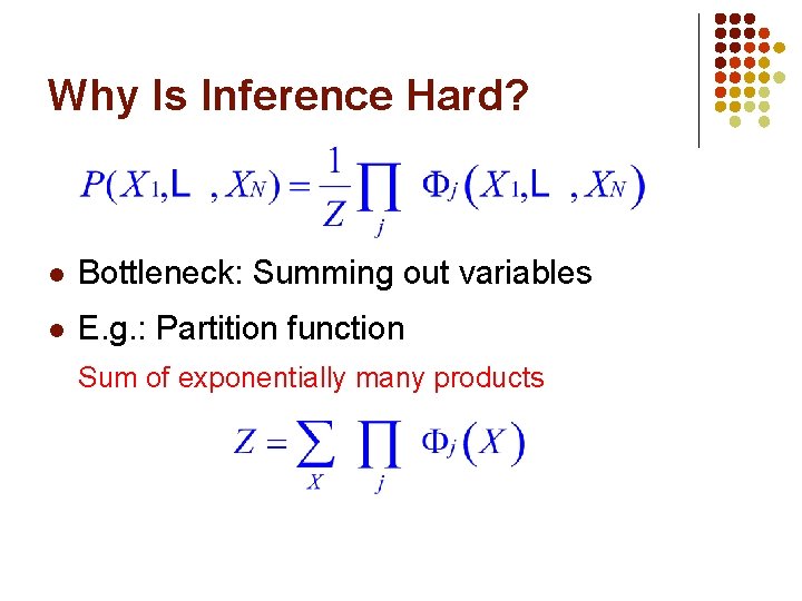
Why Is Inference Hard? l Bottleneck: Summing out variables l E. g. : Partition function Sum of exponentially many products

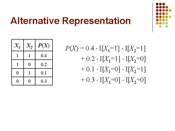
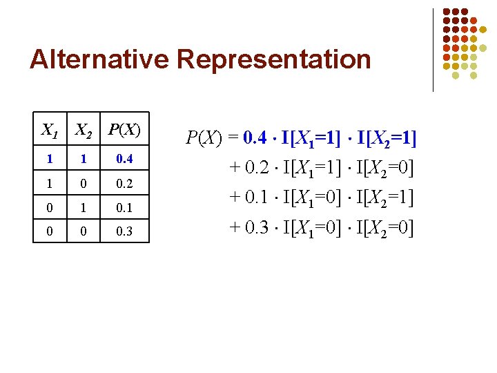
Alternative Representation X 1 X 2 P(X) 1 1 0. 4 1 0 0. 2 0 1 0 0 0. 3 P(X) = 0. 4 I[X 1=1] I[X 2=1] + 0. 2 I[X 1=1] I[X 2=0] + 0. 1 I[X 1=0] I[X 2=1] + 0. 3 I[X 1=0] I[X 2=0]

Alternative Representation X 1 X 2 P(X) 1 1 0. 4 1 0 0. 2 0 1 0 0 0. 3 P(X) = 0. 4 I[X 1=1] I[X 2=1] + 0. 2 I[X 1=1] I[X 2=0] + 0. 1 I[X 1=0] I[X 2=1] + 0. 3 I[X 1=0] I[X 2=0]

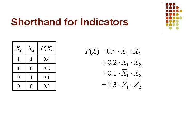
Shorthand for Indicators X 1 X 2 P(X) 1 1 0. 4 1 0 0. 2 0 1 0 0 0. 3 P(X) = 0. 4 X 1 X 2 + 0. 2 X 1 X 2 + 0. 3 X 1 X 2

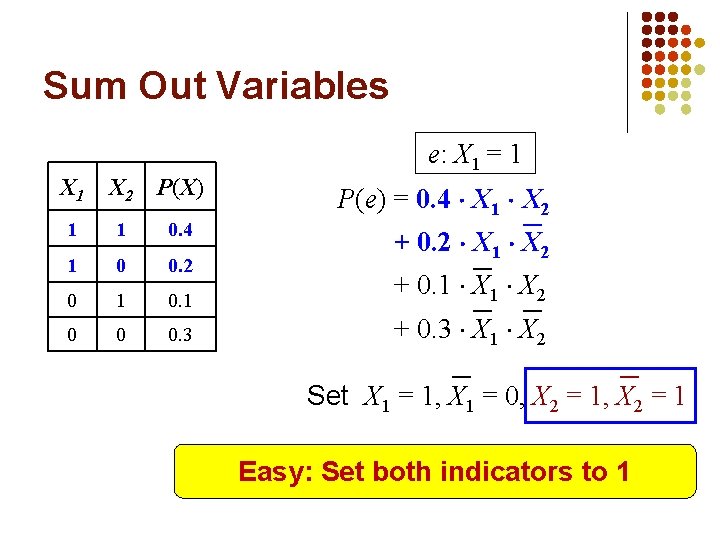
Sum Out Variables e: X 1 = 1 X 2 P(X) 1 1 0. 4 1 0 0. 2 0 1 0 0 0. 3 P(e) = 0. 4 X 1 X 2 + 0. 2 X 1 X 2 + 0. 3 X 1 X 2 Set X 1 = 1, X 1 = 0, X 2 = 1 Easy: Set both indicators to 1

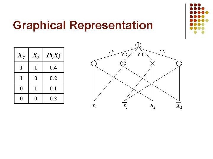
Graphical Representation X 1 X 2 P(X) 1 1 0. 4 1 0 0. 2 0 1 0 0 0. 3 0. 4 X 1 0. 2 X 1 0. 3 0. 1 X 2

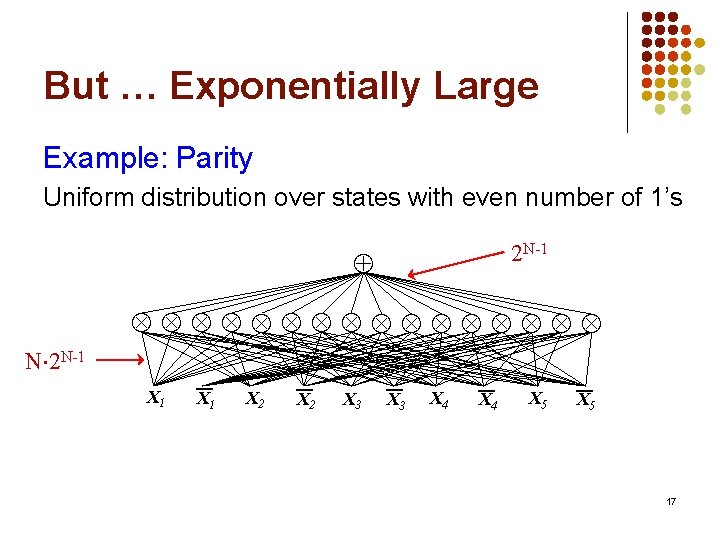
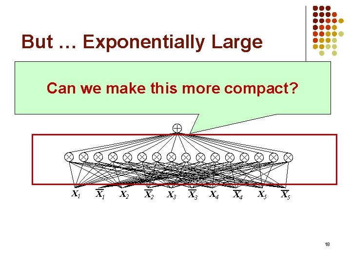
But … Exponentially Large Example: Parity Uniform distribution over states with even number of 1’s 2 N-1 N 2 N-1 X 1 X 2 X 3 X 4 X 5 17

But … Exponentially Large Example: Parity Can we make this more compact? Uniform distribution over states of even number of 1’s X 1 X 2 X 3 X 4 X 5 18

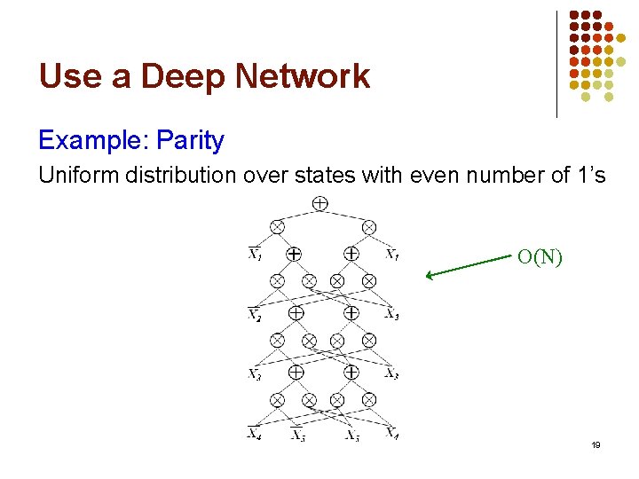
Use a Deep Network Example: Parity Uniform distribution over states with even number of 1’s O(N) 19

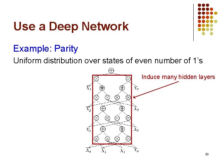
Use a Deep Network Example: Parity Uniform distribution over states of even number of 1’s Induce many hidden layers 20

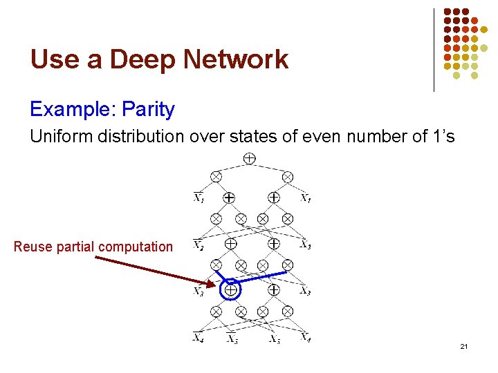
Use a Deep Network Example: Parity Uniform distribution over states of even number of 1’s Reuse partial computation 21

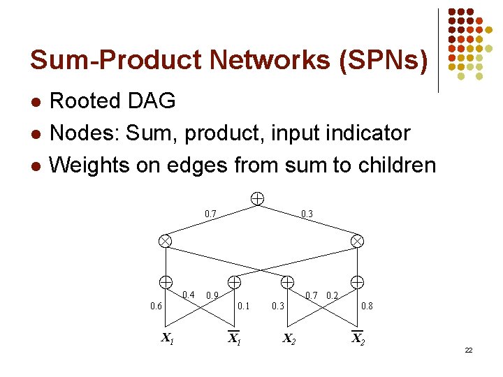
Sum-Product Networks (SPNs) l l l Rooted DAG Nodes: Sum, product, input indicator Weights on edges from sum to children 0. 7 0. 3 0. 6 X 1 0. 4 0. 9 0. 1 X 1 0. 3 X 2 0. 7 0. 2 0. 8 X 2 22

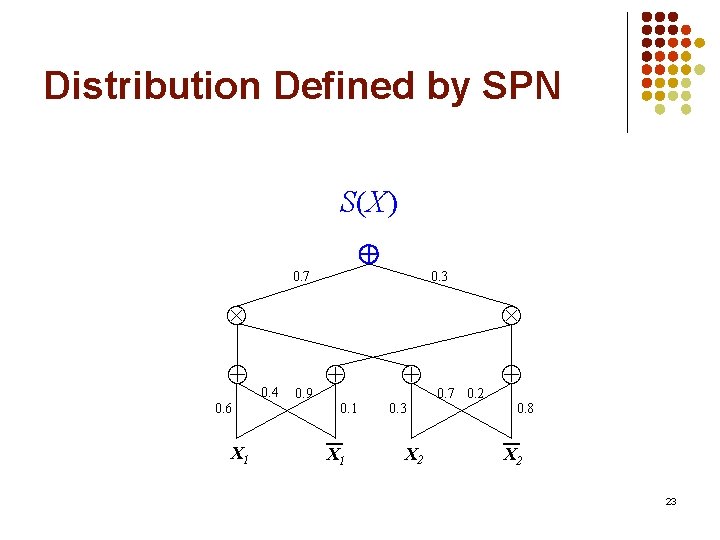
Distribution Defined by SPN P(X) S(X) 0. 7 0. 3 0. 6 X 1 0. 4 0. 9 0. 1 X 1 0. 3 X 2 0. 7 0. 2 0. 8 X 2 23

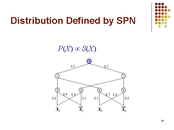
Distribution Defined by SPN P(X) S(X) 0. 7 0. 3 0. 6 X 1 0. 4 0. 9 0. 1 X 1 0. 3 X 2 0. 7 0. 2 0. 8 X 2 24

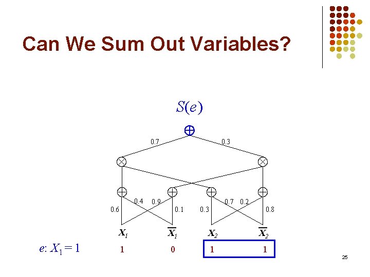
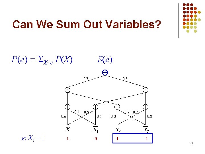
Can We Sum Out Variables? P(e) X e S(X) S(e) 0. 7 0. 3 0. 6 e: X 1 = 1 0. 4 0. 9 0. 1 X 1 1 0. 3 0. 7 0. 2 0. 8 X 1 X 2 0 1 1 25

Can We Sum Out Variables? P(e) = X e P(X) S(e) 0. 7 0. 3 0. 6 e: X 1 = 1 0. 4 0. 9 0. 1 X 1 1 0. 3 0. 7 0. 2 0. 8 X 1 X 2 0 1 1 26

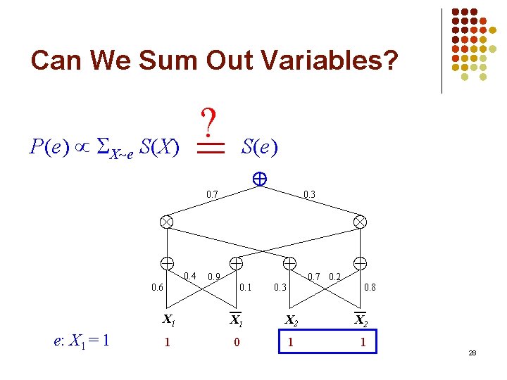
Can We Sum Out Variables? P(e) X e S(X) S(e) 0. 7 0. 3 0. 6 e: X 1 = 1 0. 4 0. 9 0. 1 X 1 1 0. 3 0. 7 0. 2 0. 8 X 1 X 2 0 1 1 27

Can We Sum Out Variables? ? = P(e) X e S(X) S(e) 0. 7 0. 3 0. 6 e: X 1 = 1 0. 4 0. 9 0. 1 X 1 1 0. 3 0. 7 0. 2 0. 8 X 1 X 2 0 1 1 28

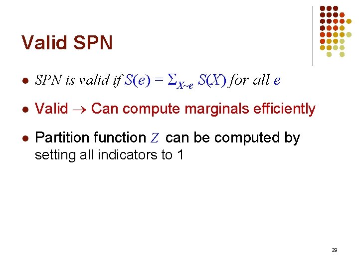
Valid SPN l SPN is valid if S(e) = X e S(X) for all e l Valid Can compute marginals efficiently l Partition function Z can be computed by setting all indicators to 1 29

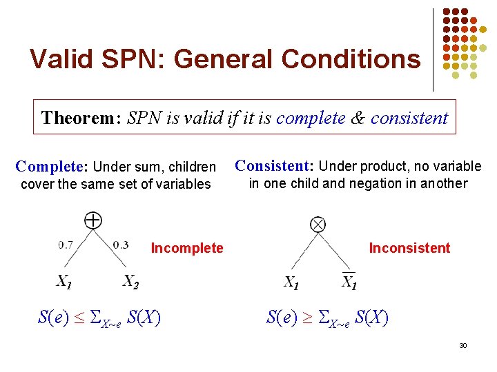
Valid SPN: General Conditions Theorem: SPN is valid if it is complete & consistent Complete: Under sum, children Consistent: Under product, no variable cover the same set of variables in one child and negation in another Incomplete S(e) X e S(X) Inconsistent S(e) X e S(X) 30

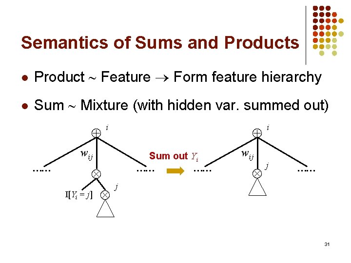
Semantics of Sums and Products l Product Feature Form feature hierarchy l Sum Mixture (with hidden var. summed out) i wij …… Sum out Yi I[Yi = j] …… j …… wij i j …… 31

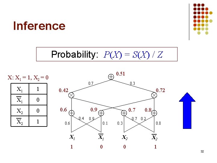
Inference Probability: P(X) = S(X) / Z X: X 1 = 1, X 2 = 0 X 1 1 X 1 0 X 2 1 0. 51 0. 7 0. 3 0. 42 0. 72 0. 6 0. 9 0. 4 0. 9 0. 1 0. 3 0. 7 0. 8 0. 7 0. 2 0. 8 X 1 X 2 1 0 0 1 32

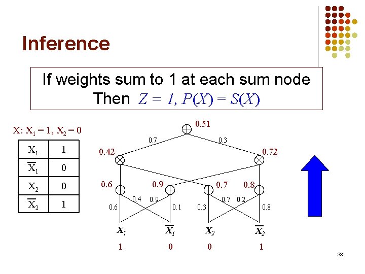
Inference If weights sum to 1 at each sum node Then Z = 1, P(X) = S(X) X: X 1 = 1, X 2 = 0 X 1 1 X 1 0 X 2 1 0. 51 0. 7 0. 3 0. 42 0. 72 0. 6 0. 9 0. 4 0. 9 0. 1 0. 3 0. 7 0. 8 0. 7 0. 2 0. 8 X 1 X 2 1 0 0 1 33

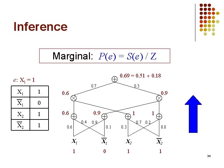
Inference Marginal: P(e) = S(e) / Z e: X 1 = 1 X 1 0 X 2 1 0. 7 0. 69 = 0. 51 0. 18 0. 3 0. 9 0. 6 0. 9 0. 4 0. 9 0. 1 0. 3 1 1 0. 7 0. 2 0. 8 X 1 X 2 1 0 1 1 34

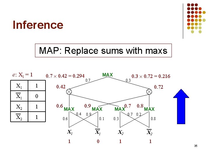
Inference MAP: Replace sums with maxs e: X 1 = 1 X 1 0. 7 0. 42 = 0. 294 1 X 1 0 X 2 1 0. 42 0. 6 MAX 0. 7 0. 3 0. 72 = 0. 216 0. 9 MAX 0. 4 0. 6 MAX 0. 7 MAX 0. 9 0. 8 0. 72 MAX 0. 7 0. 2 0. 1 0. 3 0. 8 X 1 X 2 1 0 1 1 35

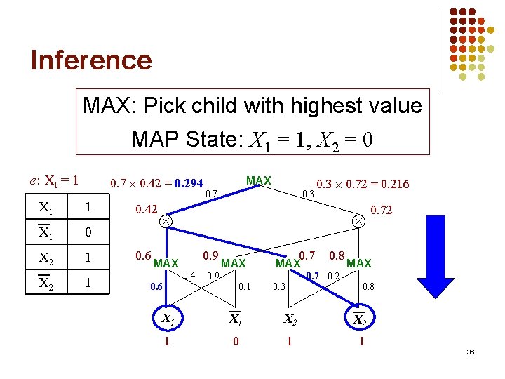
Inference MAX: Pick child with highest value MAP State: X 1 = 1, X 2 = 0 e: X 1 = 1 X 1 0. 7 0. 42 = 0. 294 1 X 1 0 X 2 1 0. 42 0. 6 MAX 0. 7 0. 3 0. 72 = 0. 216 0. 9 MAX 0. 4 0. 6 MAX 0. 7 MAX 0. 9 0. 8 0. 72 MAX 0. 7 0. 2 0. 1 0. 3 0. 8 X 1 X 2 1 0 1 1 36

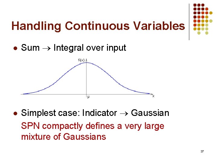
Handling Continuous Variables l l Sum Integral over input Simplest case: Indicator Gaussian SPN compactly defines a very large mixture of Gaussians 37

SPNs Everywhere l Graphical models Existing tractable models, e. g. : hierarchical mixture model, thin junction tree, etc. SPNs can compactly represent many more distributions 38

SPNs Everywhere l Graphical models Inference methods, e. g. : Junction-tree algorithm, message passing, … SPNs can represent, combine, and learn the optimal way 39

SPNs Everywhere l Graphical models SPNs can be more compact by leveraging determinism, context-specific independence, etc. 40

SPNs Everywhere l Graphical models l Models for efficient inference E. g. , arithmetic circuits, AND/OR graphs, case-factor diagrams SPN: First approach for learning directly from data 41

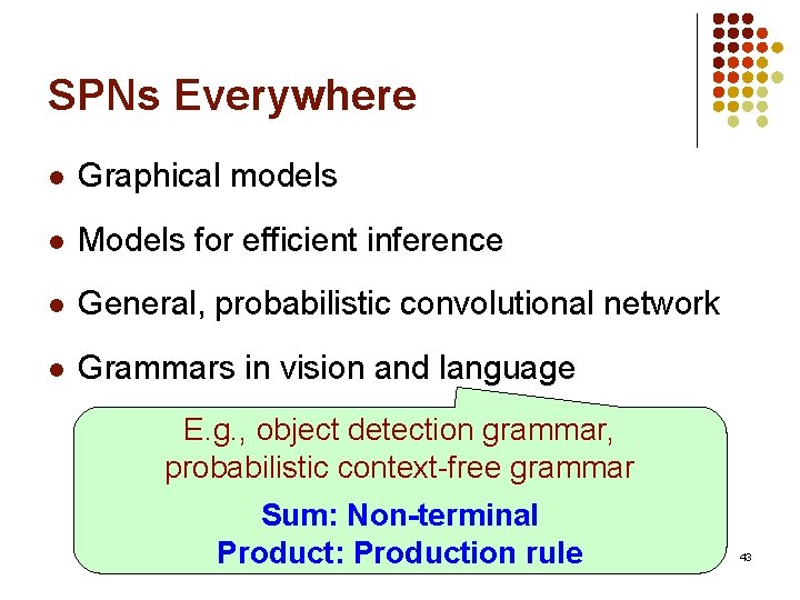
SPNs Everywhere l Graphical models l Models for efficient inference l General, probabilistic convolutional network Sum: Average-pooling Max: Max-pooling 42

SPNs Everywhere l Graphical models l Models for efficient inference l General, probabilistic convolutional network l Grammars in vision and language E. g. , object detection grammar, probabilistic context-free grammar Sum: Non-terminal Product: Production rule 43

Outline l l Sum-product networks (SPNs) Learning SPNs Experimental results Conclusion 44

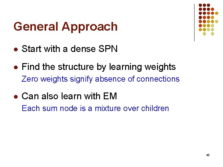
General Approach l Start with a dense SPN l Find the structure by learning weights Zero weights signify absence of connections l Can also learn with EM Each sum node is a mixture over children 45

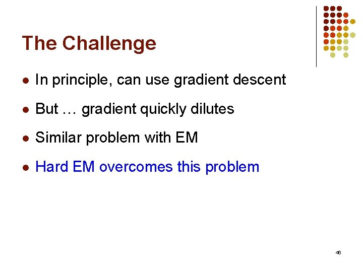
The Challenge l In principle, can use gradient descent l But … gradient quickly dilutes l Similar problem with EM l Hard EM overcomes this problem 46

Our Learning Algorithm l Online learning Hard EM l Sum node maintains counts for each child l For each example l l Find MAP instantiation with current weights Increment count for each chosen child Renormalize to set new weights Repeat until convergence 47

Outline l l Sum-product networks (SPNs) Learning SPNs Experimental results Conclusion 48

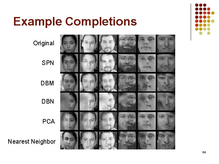
Task: Image Completion l Very challenging l Good for evaluating deep models l Methodology: l l l Learn a model from training images Complete unseen test images Measure mean square errors 49

Datasets l Main evaluation: Caltech-101 [Fei-Fei et al. , 2004] l l 101 categories, e. g. , faces, cars, elephants Each category: 30 – 800 images l Also, Olivetti [Samaria & Harter, 1994] (400 faces) l Each category: Last third for test Test images: Unseen objects 50

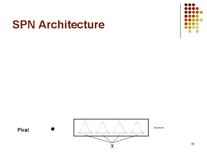
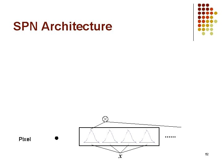
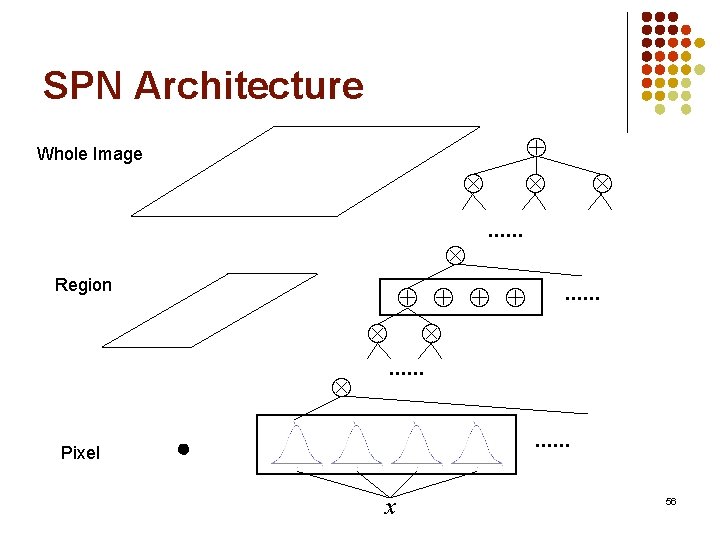
SPN Architecture Pixel . . . x 51

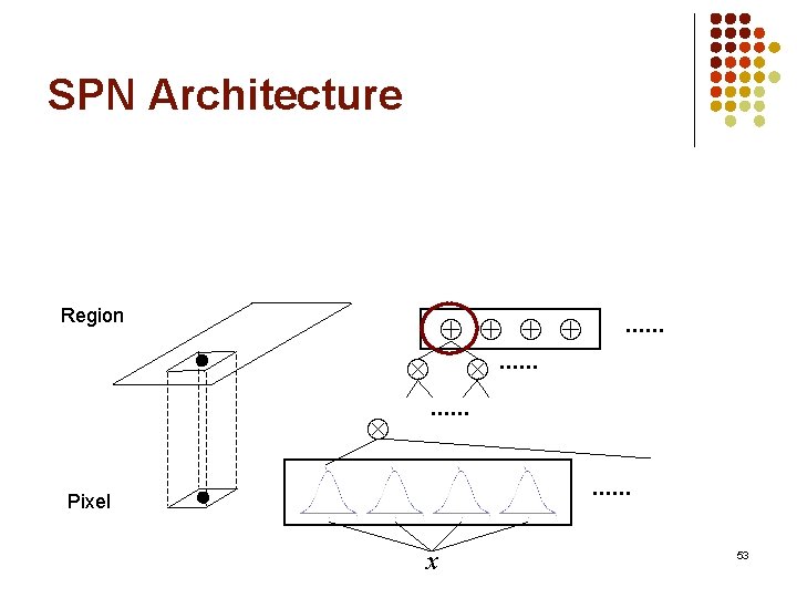
SPN Architecture Pixel . . . x 52

SPN Architecture Region . . . Pixel . . . . x 53

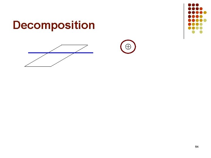
Decomposition 54

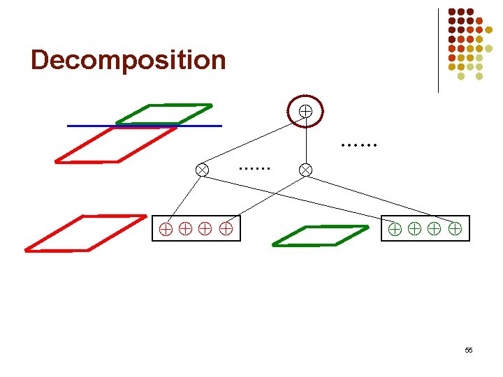
Decomposition …… 55

SPN Architecture Whole Image . . . Region Pixel . . . . x 56

Systems l SPN l DBM [Salakhutdinov & Hinton, 2010] l DBN [Hinton & Salakhutdinov, 2006] l PCA [Turk & Pentland, 1991] l Nearest neighbor [Hays & Efros, 2007] 57

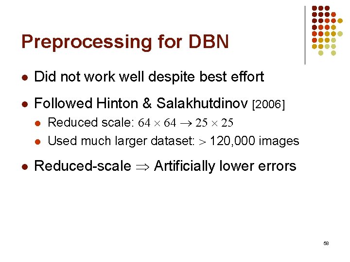
Preprocessing for DBN l Did not work well despite best effort l Followed Hinton & Salakhutdinov [2006] l l l Reduced scale: 64 25 Used much larger dataset: 120, 000 images Reduced-scale Artificially lower errors 58

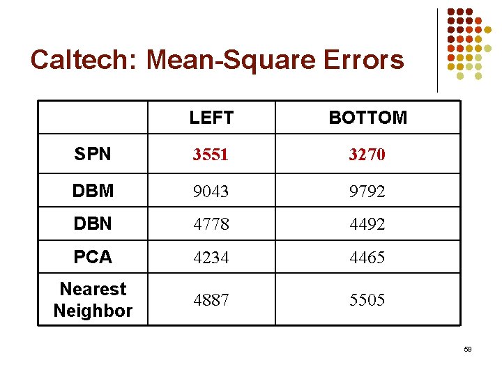
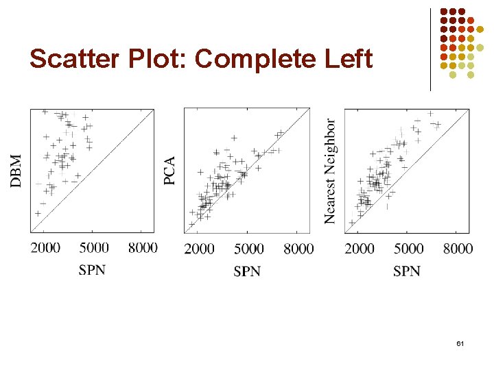
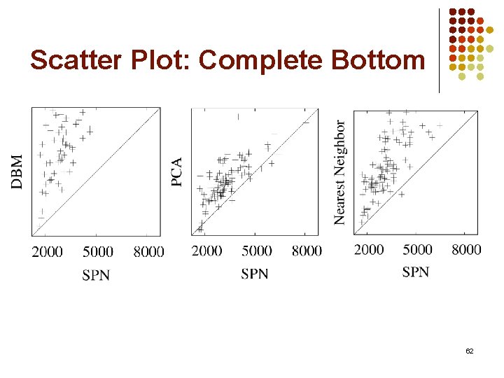
Caltech: Mean-Square Errors LEFT BOTTOM SPN 3551 3270 DBM 9043 9792 DBN 4778 4492 PCA 4234 4465 Nearest Neighbor 4887 5505 59

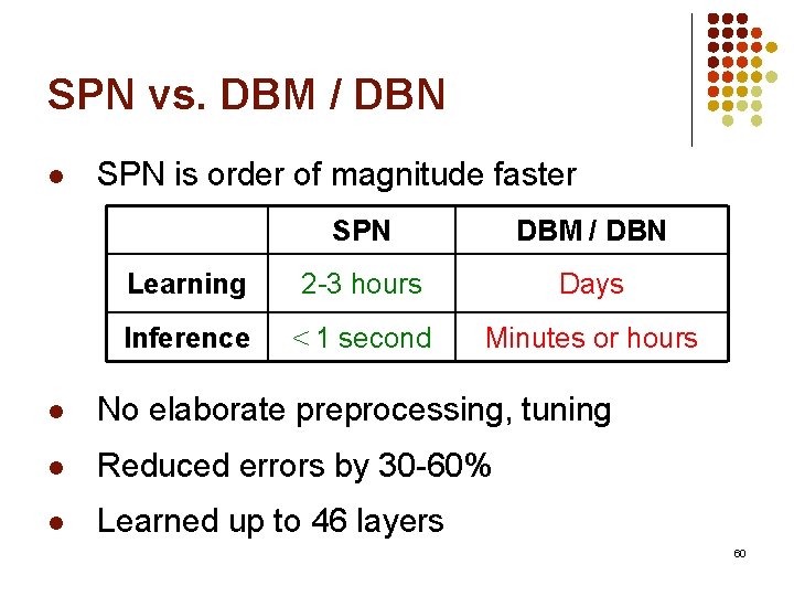
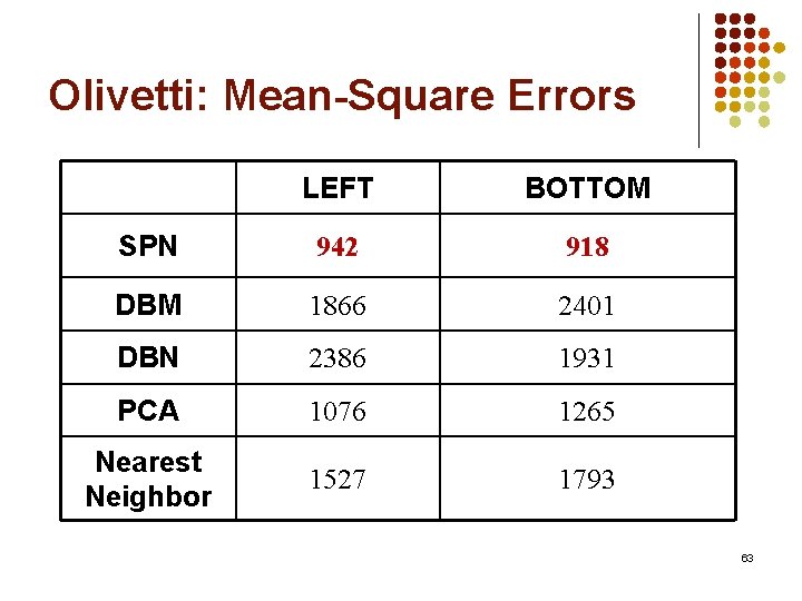
SPN vs. DBM / DBN l SPN is order of magnitude faster SPN DBM / DBN Learning 2 -3 hours Days Inference < 1 second Minutes or hours l No elaborate preprocessing, tuning l Reduced errors by 30 -60% l Learned up to 46 layers 60

Scatter Plot: Complete Left 61

Scatter Plot: Complete Bottom 62

Olivetti: Mean-Square Errors LEFT BOTTOM SPN 942 918 DBM 1866 2401 DBN 2386 1931 PCA 1076 1265 Nearest Neighbor 1527 1793 63

Example Completions Original SPN DBM DBN PCA Nearest Neighbor 64

Open Questions l Other learning algorithms l Discriminative learning l Architecture l Continuous SPNs l Sequential domains l Other applications 65

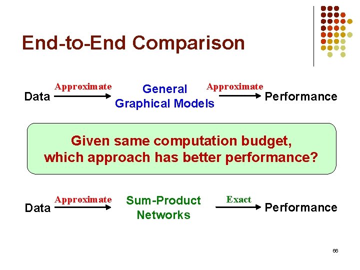
End-to-End Comparison Data Approximate General Performance Graphical Models Given same computation budget, which approach has better performance? Data Approximate Sum-Product Networks Exact Performance 66

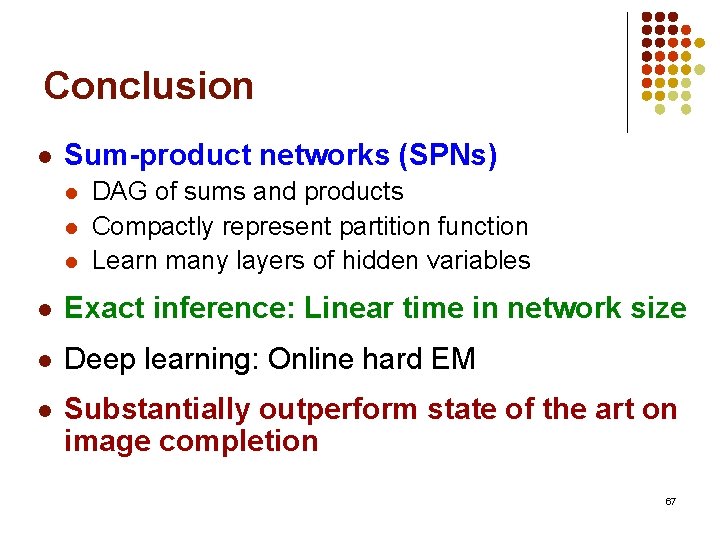
Conclusion l Sum-product networks (SPNs) l l l DAG of sums and products Compactly represent partition function Learn many layers of hidden variables l Exact inference: Linear time in network size l Deep learning: Online hard EM l Substantially outperform state of the art on image completion 67