Summary of lecture 7 Error detection schemes arise

Summary of lecture 7 • Error detection schemes arise in a range of different places, such as • Travelers Checks • airline tickets • bank account numbers • universal product codes (barcodes) • ISBNs • Zip codes. • In these cases, check digits are used to ensure that codes are correct. • If an error arises we are able to correct the error manually.

MAT 199: Math Alive Birth, Growth, Death and Chaos Ian Griffiths Mathematical Institute, University of Oxford, Department of Mathematics, Princeton University

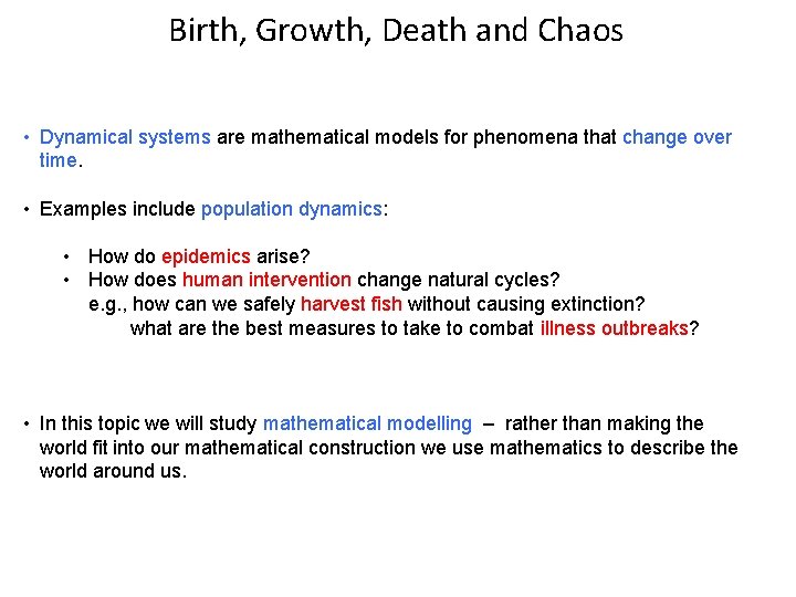
Birth, Growth, Death and Chaos • Dynamical systems are mathematical models for phenomena that change over time.

Birth, Growth, Death and Chaos • Dynamical systems are mathematical models for phenomena that change over time. • Examples include population dynamics: • How do epidemics arise? • How does human intervention change natural cycles? e. g. , how can we safely harvest fish without causing extinction? what are the best measures to take to combat illness outbreaks?

Birth, Growth, Death and Chaos • Dynamical systems are mathematical models for phenomena that change over time. • Examples include population dynamics: • How do epidemics arise? • How does human intervention change natural cycles? e. g. , how can we safely harvest fish without causing extinction? what are the best measures to take to combat illness outbreaks? • In this topic we will study mathematical modelling – rather than making the world fit into our mathematical construction we use mathematics to describe the world around us.

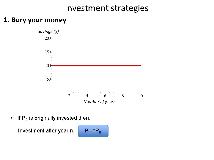
Investment strategies 1. Bury your money Savings ($) Number of years • If P 0 is originally invested then: Investment after year n, Pn =P 0

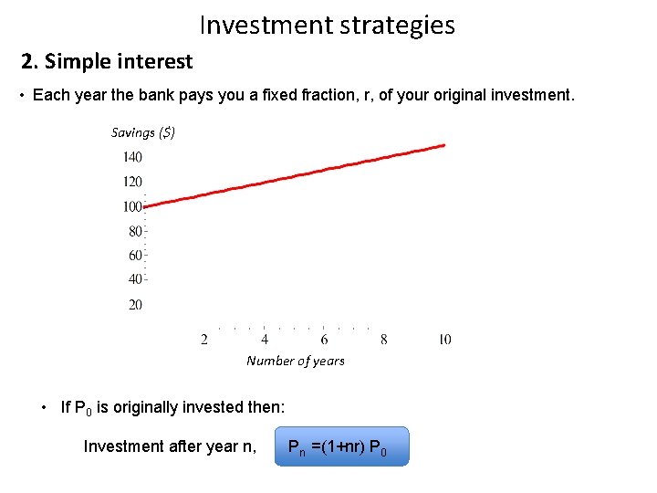
Investment strategies 2. Simple interest • Each year the bank pays you a fixed fraction, r, of your original investment. Savings ($) Number of years • If P 0 is originally invested then: Investment after year n, Pn =(1+nr) P 0

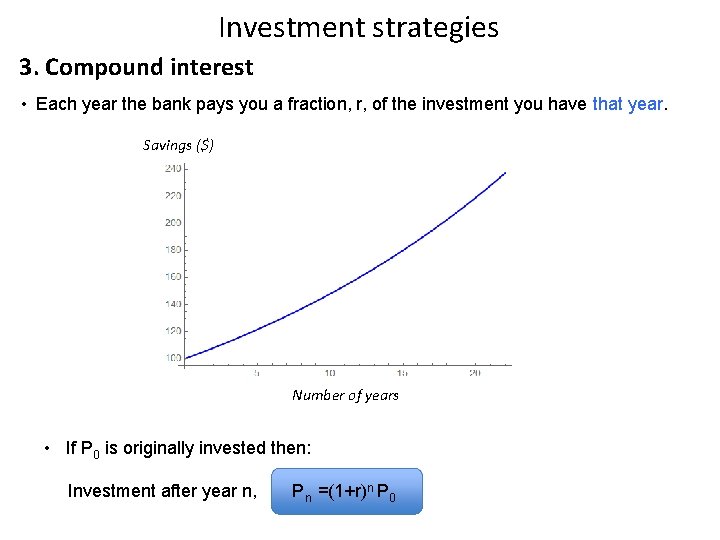
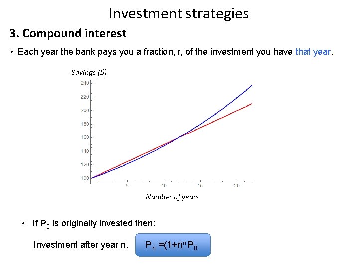
Investment strategies 3. Compound interest • Each year the bank pays you a fraction, r, of the investment you have that year. Savings ($) Number of years • If P 0 is originally invested then: Investment after year n, Pn =(1+r)n P 0

Investment strategies 3. Compound interest • Each year the bank pays you a fraction, r, of the investment you have that year. Savings ($) Number of years • If P 0 is originally invested then: Investment after year n, Pn =(1+r)n P 0

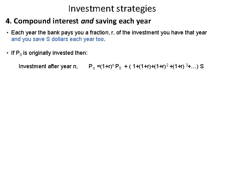
Investment strategies 4. Compound interest and saving each year • Each year the bank pays you a fraction, r, of the investment you have that year and you save S dollars each year too. • If P 0 is originally invested then: Investment after year n, Pn =(1+r)n P 0 + ( 1+(1+r)2 +(1+r) 3+…) S

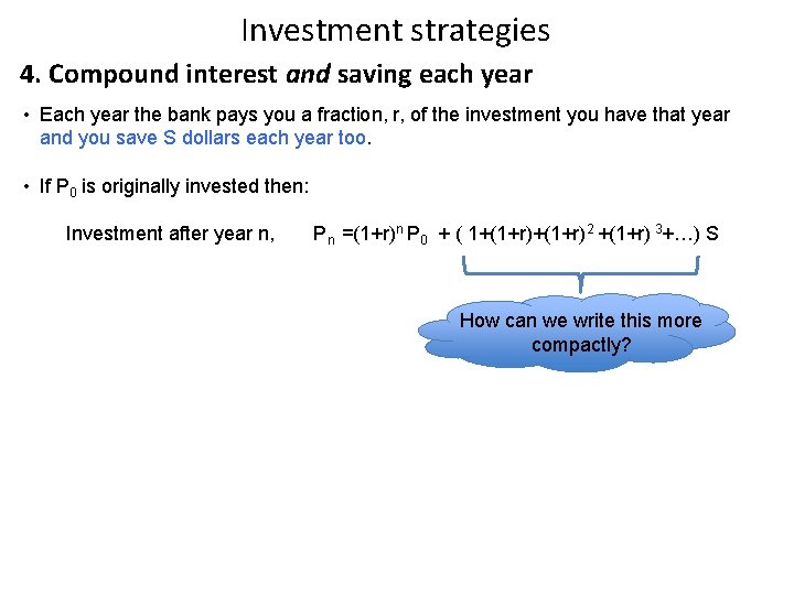
Investment strategies 4. Compound interest and saving each year • Each year the bank pays you a fraction, r, of the investment you have that year and you save S dollars each year too. • If P 0 is originally invested then: Investment after year n, Pn =(1+r)n P 0 + ( 1+(1+r)2 +(1+r) 3+…) S How can we write this more compactly?

Summary of lecture 8 • Mathematical modelling is used to describe and understand the world around us. • Dynamical systems are mathematical models for phenomena that change over time. • We can write down rules that tell us what state we are in at any given time, e. g. , the amount of savings we have in a bank account at any given time. • It is easy to work out the state we will be in at the next step (e. g. , the money we have in our account next year) given the current state. • It is helpful if we can obtain expressions for the state we will be in at any time in terms of the original state.

Carl Friedrich Gauss 1777 – 1855

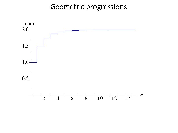
Geometric progressions

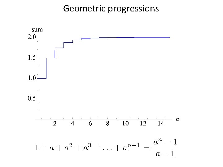
Geometric progressions

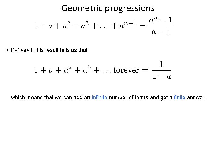
Geometric progressions • If -1<a<1 this result tells us that which means that we can add an infinite number of terms and get a finite answer.

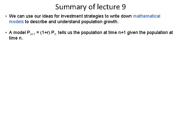
Summary of lecture 9 • We can use our ideas for investment strategies to write down mathematical models to describe and understand population growth. • A model Pn+1 = (1+r) Pn tells us the population at time n+1 given the population at time n.

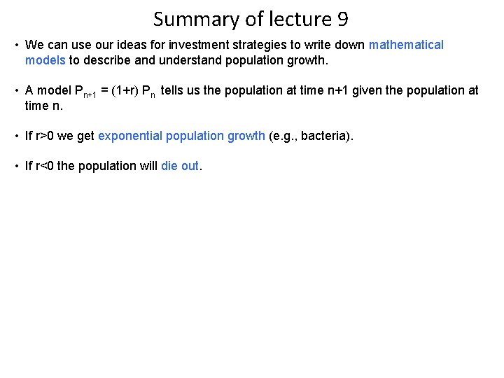
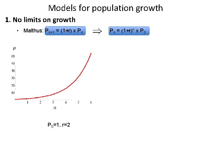
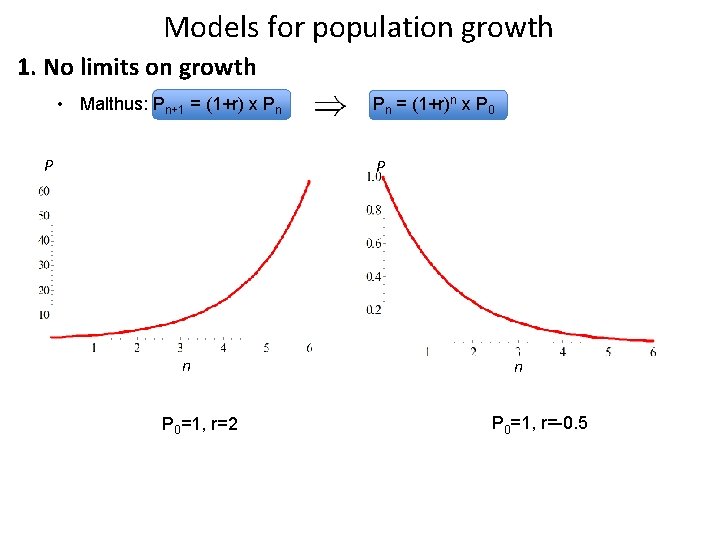
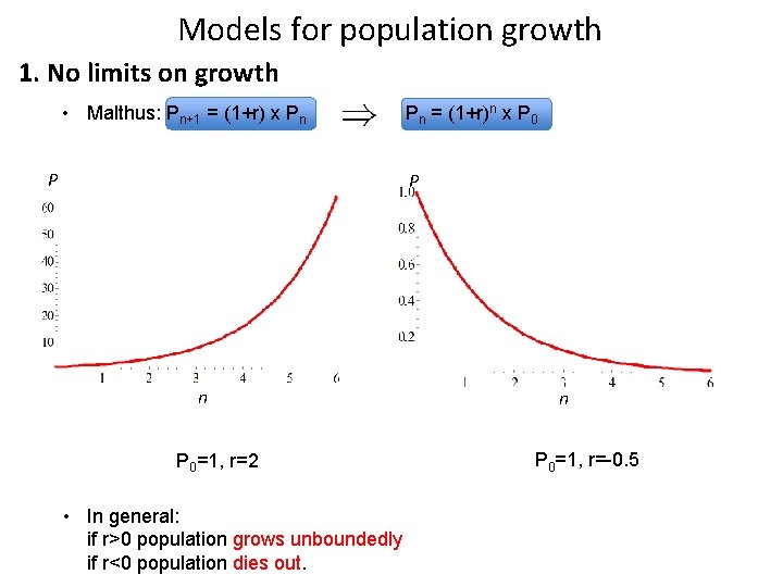
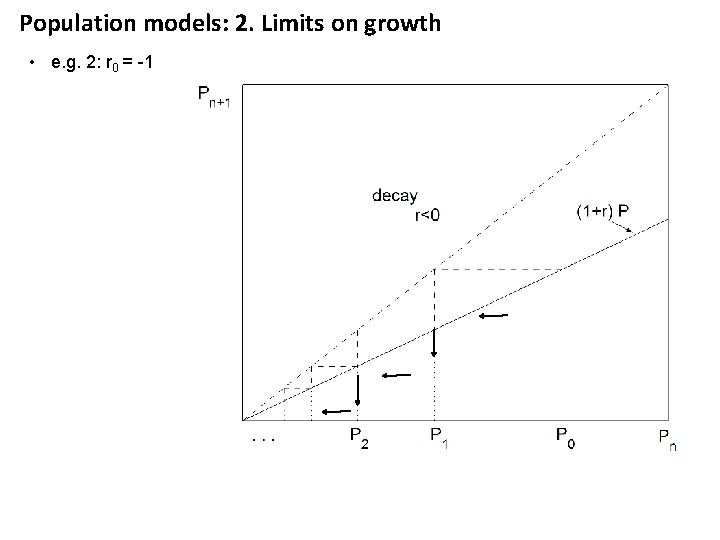
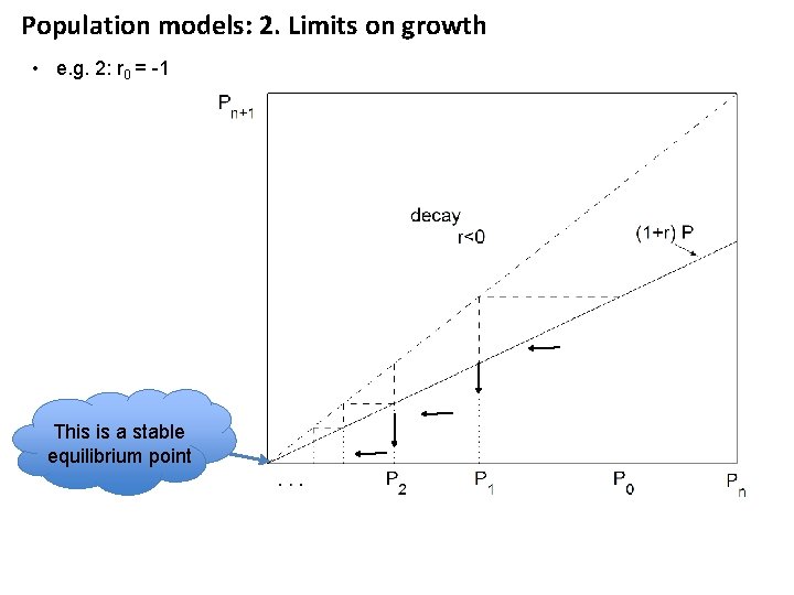
Summary of lecture 9 • We can use our ideas for investment strategies to write down mathematical models to describe and understand population growth. • A model Pn+1 = (1+r) Pn tells us the population at time n+1 given the population at time n. • If r>0 we get exponential population growth (e. g. , bacteria). • If r<0 the population will die out.

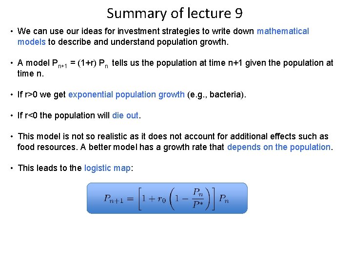
Summary of lecture 9 • We can use our ideas for investment strategies to write down mathematical models to describe and understand population growth. • A model Pn+1 = (1+r) Pn tells us the population at time n+1 given the population at time n. • If r>0 we get exponential population growth (e. g. , bacteria). • If r<0 the population will die out. • This model is not so realistic as it does not account for additional effects such as food resources. A better model has a growth rate that depends on the population. • This leads to the logistic map:

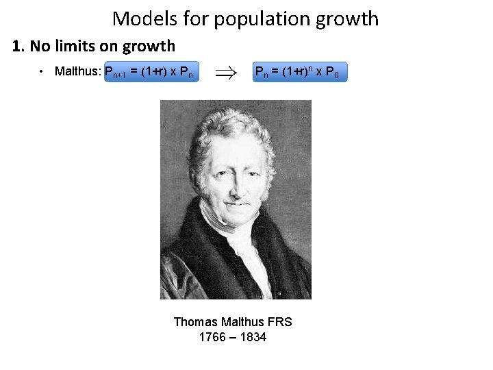
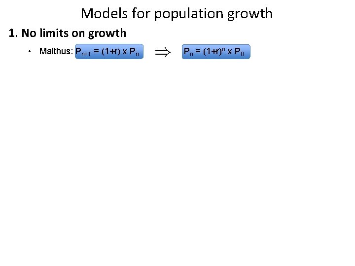
Models for population growth 1. No limits on growth • Malthus: Pn+1 = (1+r) x Pn Pn = (1+r)n x P 0 Thomas Malthus FRS 1766 – 1834

Models for population growth 1. No limits on growth • Malthus: Pn+1 = (1+r) x Pn Pn = (1+r)n x P 0

Models for population growth 1. No limits on growth • Malthus: Pn+1 = (1+r) x Pn P 0=1, r=2 Pn = (1+r)n x P 0

Models for population growth 1. No limits on growth • Malthus: Pn+1 = (1+r) x Pn P Pn = (1+r)n x P 0 P n P 0=1, r=2 n P 0=1, r=-0. 5

Models for population growth 1. No limits on growth • Malthus: Pn+1 = (1+r) x Pn P Pn = (1+r)n x P 0 P n P 0=1, r=2 • In general: if r>0 population grows unboundedly if r<0 population dies out. n P 0=1, r=-0. 5

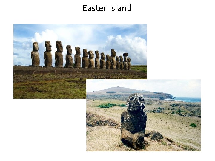
Easter Island

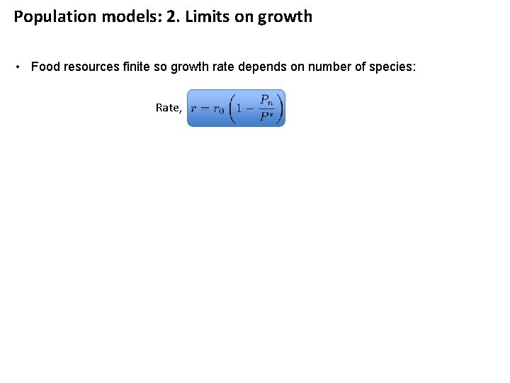
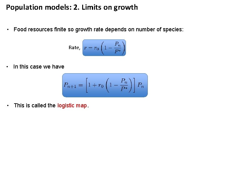
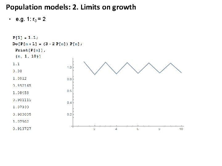
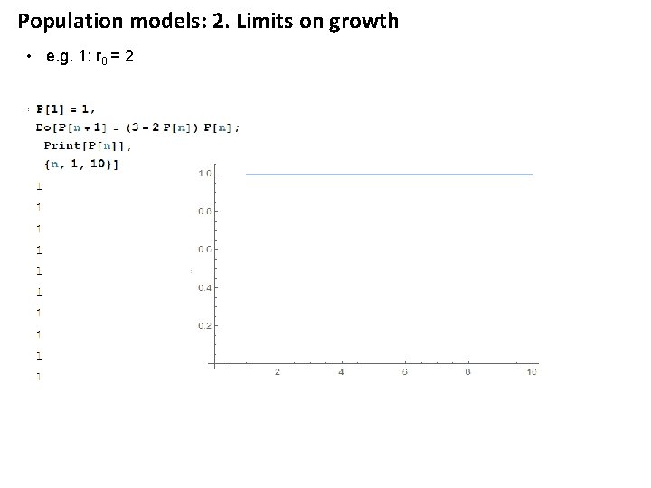
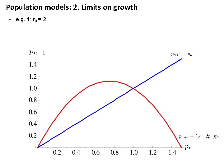
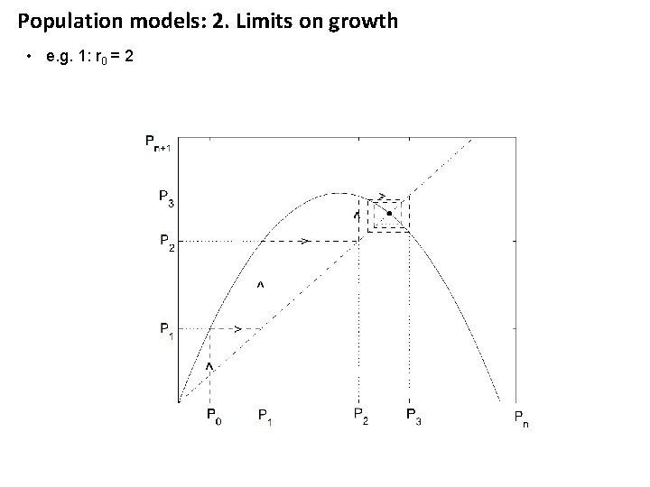
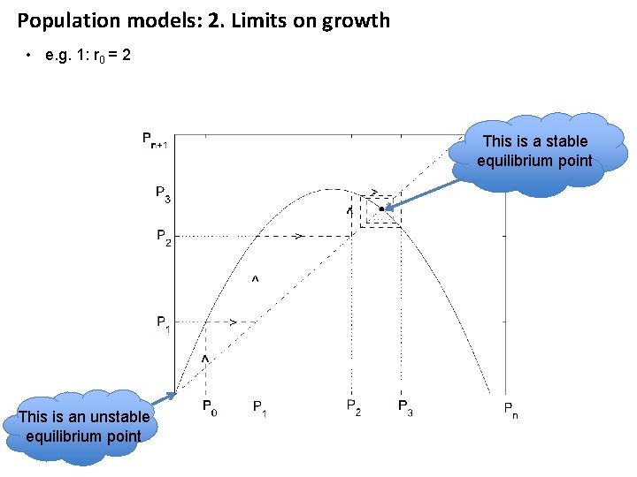
Population models: 2. Limits on growth • Food resources finite so growth rate depends on number of species: Rate,

Population models: 2. Limits on growth • Food resources finite so growth rate depends on number of species: Rate, • In this case we have • This is called the logistic map.

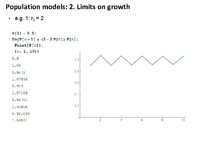
Population models: 2. Limits on growth • e. g. 1: r 0 = 2

Population models: 2. Limits on growth • e. g. 1: r 0 = 2

Population models: 2. Limits on growth • e. g. 1: r 0 = 2

Population models: 2. Limits on growth • e. g. 1: r 0 = 2

Population models: 2. Limits on growth • e. g. 1: r 0 = 2

Population models: 2. Limits on growth • e. g. 1: r 0 = 2 This is a stable equilibrium point This is an unstable equilibrium point

Population models: 2. Limits on growth • e. g. 2: r 0 = -1

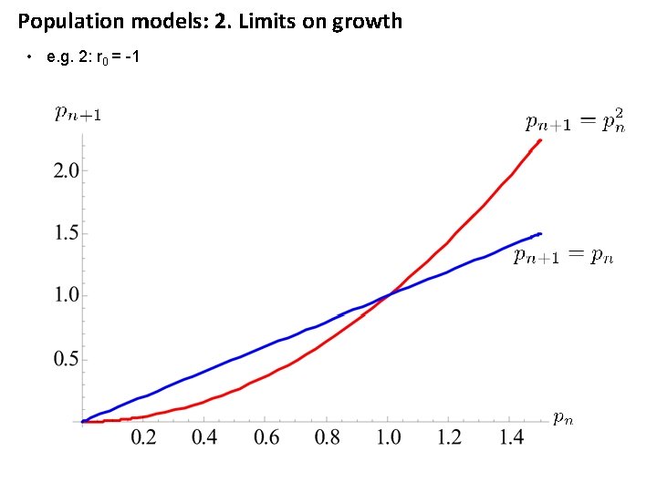
Population models: 2. Limits on growth • e. g. 2: r 0 = -1

Population models: 2. Limits on growth • e. g. 2: r 0 = -1 This is a stable equilibrium point

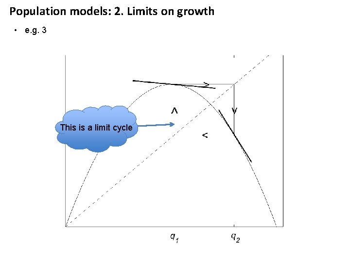
Population models: 2. Limits on growth • e. g. 3 This is a limit cycle

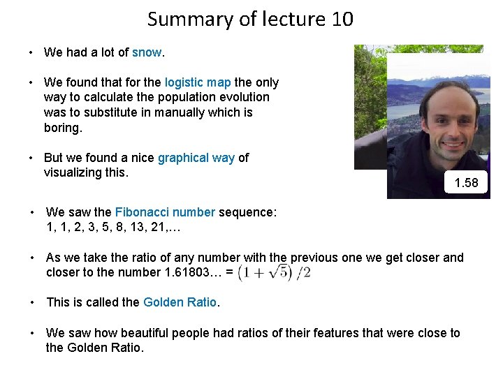
Summary of lecture 10 • We had a lot of snow. • We found that for the logistic map the only way to calculate the population evolution was to substitute in manually which is boring. • But we found a nice graphical way of visualizing this. 1. 45 1. 58 • We saw the Fibonacci number sequence: 1, 1, 2, 3, 5, 8, 13, 21, … • As we take the ratio of any number with the previous one we get closer and closer to the number 1. 61803… = • This is called the Golden Ratio. • We saw how beautiful people had ratios of their features that were close to the Golden Ratio.

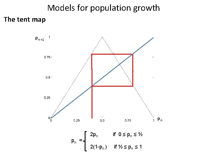
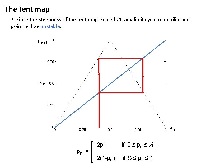
Models for population growth The tent map pn +1 pn pn = 2 pn if 0 ≤ pn ≤ ½ 2(1 -pn ) if ½ ≤ pn ≤ 1

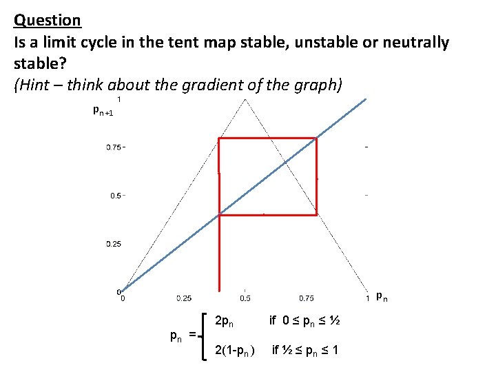
Question Is a limit cycle in the tent map stable, unstable or neutrally stable? (Hint – think about the gradient of the graph) pn +1 pn pn = 2 pn if 0 ≤ pn ≤ ½ 2(1 -pn ) if ½ ≤ pn ≤ 1

The tent map • Since the steepness of the tent map exceeds 1, any limit cycle or equilibrium point will be unstable. pn +1 pn pn = 2 pn if 0 ≤ pn ≤ ½ 2(1 -pn ) if ½ ≤ pn ≤ 1

Summary of lecture 11 Stability of equilibrium points • If the steepness (positive or negative) of the population graph is less than 1 at an equilibrium point then the equilibrium point is stable. • If the steepness (positive or negative) of the population graph exceeds 1 at an equilibrium point then the equilibrium point is unstable. • We can have limit cycles when the steepness (positive or negative) of the population graph equals 1. • We can change variables to express a dynamical system in a different way. e. g. , instead of population of animals, the cost of looking after the animals.

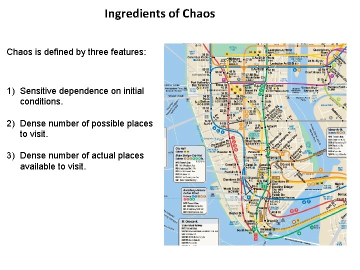
Ingredients of Chaos is defined by three features: 1) Sensitive dependence on initial conditions. 2) Dense number of possible places to visit. 3) Dense number of actual places available to visit.