Summarizing Data Statistics probability sampling inference statistics probability

Summarizing Data

Statistics

probability sampling inference statistics probability vs. statistics

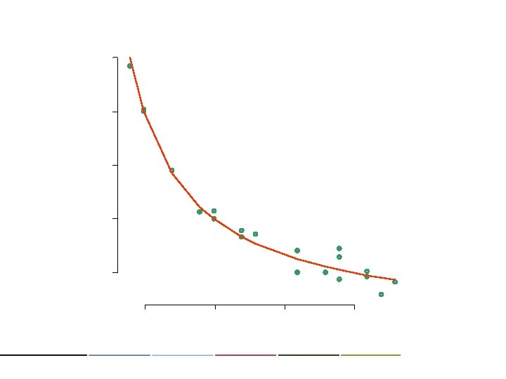
Distribution ?

Distribution : A mathematical way to represent the diversity of characteristics of a group. Group may be a sample and a population. • population distribution • distribution of a sample
")
statistics dist’n of a sample pop’n dist’n realistic imaginary data Theory (model)

Statistics starts from data.

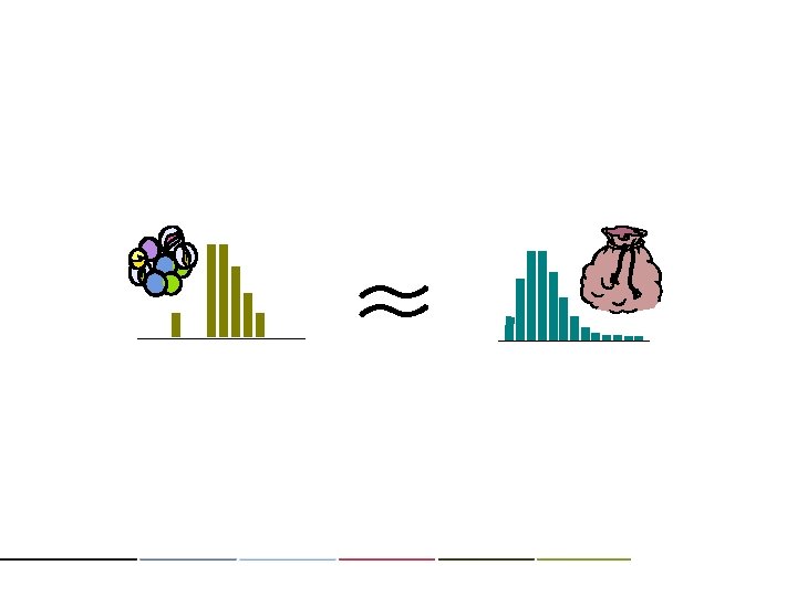
Data are not just sets of numbers. Data are clues to truth, and say about truth.

The 1 st principle of statistics : The sample is not the same with the population, but the population is represented by the sample sufficiently well.

Datawork

Woodwork & Datawork • From forest • From real world • Making timber • Data collecting • Inspecting wood grain • Exploring data • Cutting • Reducing data • Structuring • Modeling • Finishing • Evaluating

Craft & Endeavor

Tools & Skills
 • Minitab, SPSS,")
Statistical tools • Paper, pencil & calculator • Spreadsheet SW (Excel) • Minitab, SPSS, SAS, R • DBMS ( Access, Oracle, …) • C/C++, Java, Python, … You need skill to use these.

Also, you need craft & experiences. However, the more important point in datawork is trying to get perspectives of the data on your hand.

No typical ways for good datawork. Think, think and think ! That’s the only way.


Wood grain ?

Grain of data ?

Seeing the grain of data ≈ Exploratory Data Analysis
 The step to check the basic properties of data, by")
Exploratory Data Analysis (EDA) The step to check the basic properties of data, by using the basic statistical methods. From EDA, we aim to develop insight on data, as a first step for more specific analysis.
 • bar")
Basic Statistical Methods Qualitative variable • frequency table • crosstabulation (contingency table) • bar chart, pie chart, ….
 frequency distribution • histogram • dot-plot •")
Basic Statistical Methods Quantitative scale • (cumulative) frequency distribution • histogram • dot-plot • stem & leaf diagram • scatter plot • box plot, ….

Example Data Credit_Card_Bank: p 22 of SVV • 12 var’s & 100 obs’s • Many types of ‘offer’ to cardholders • To find the type of ‘offer’ that increases cardholder’s usage maximally.
![[1] "Offer. Status" (Categorical) [2] "Charges. Aug. 2008" (Quantitative) [3] "Charges. Sept. 2008" (Quantitative)](http://slidetodoc.com/presentation_image_h2/e9c44fad367db5a168e56ffb533590d0/image-28.jpg "[1] \"Offer. Status\" (Categorical) [2] \"Charges. Aug. 2008\" (Quantitative) [3] \"Charges. Sept. 2008\" (Quantitative)")
[1] "Offer. Status" (Categorical) [2] "Charges. Aug. 2008" (Quantitative) [3] "Charges. Sept. 2008" (Quantitative) [4] "Charges. Oct. 2008“ (Quantitative) [5] "Marketing. Segment" (Categorical) [6] "Industry. Segment" (Categorical) [7] "Spendlift. After. Promotion“ (Quantitative) [8] "Pre. Promotion. Avg. Spend" (Quantitative) [9] "Post. Promotion. Avg. Spend" (Quantitative) [10] "Retail. Customer" (Yes, No) [11] "Enrolled. in. Program" (Yes, No) [12] "Spendlift. Positive" (Yes, No) data. svv<-dir("c: /temp/text") dfile. svv<-paste("c: /temp/text/", data. svv, sep="") dsv<- read. table(dfile. svv[1], head=TRUE, sep="t") names(dsv) oct 08<-dsv[, 4]; loct 08<-log(oct 08); xoct 08<-loct 08[oct 08>0] mseg<-dsv[, 5]; iseg<-dsv[, 6] loct 08 = log(oct 08) oct 08 mseg iseg
![log(oct 08): [1] -Inf 6. 21 [11] 5. 50 8. 00 [21] 7. 42](http://slidetodoc.com/presentation_image_h2/e9c44fad367db5a168e56ffb533590d0/image-29.jpg "log(oct 08): [1] -Inf 6. 21 [11] 5. 50 8. 00 [21] 7. 42")
log(oct 08): [1] -Inf 6. 21 [11] 5. 50 8. 00 [21] 7. 42 6. 86 [31] 6. 71 6. 12 [41] 6. 02 2. 51 [51] 5. 25 7. 85 [61] 9. 11 5. 56 [71] 6. 80 5. 72 [81] -Inf 10. 42 [91] 5. 56 7. 39 3. 96 6. 30 8. 45 -Inf 7. 20 8. 76 8. 24 7. 54 8. 73 3. 11 3. 84 3. 13 6. 12 7. 68 3. 29 7. 15 -Inf 3. 48 4. 85 3. 90 Rounded up to 2 nd decimal round(loct 08, 2) 6. 96 4. 58 5. 62 9. 08 7. 44 7. 95 7. 47 7. 57 -Inf 5. 72 6. 95 8. 89 8. 21 5. 91 5. 88 7. 13 6. 70 8. 42 6. 63 7. 10 7. 89 3. 81 6. 91 3. 42 6. 33 -Inf 7. 52 8. 16 5. 48 -Inf 7. 35 7. 00 6. 87 6. 12 6. 24 7. 13 6. 53 4. 67 4. 89 7. 58 3. 97 8. 37 7. 15 8. 05 4. 33 8. 11 8. 33 7. 16 8. 35 8. 15 5. 97 7. 85 5. 46 7. 03 5. 93 8. 05 4. 63 5. 61 4. 65 6. 30 log(0) = - Inf
![Sorted values of log(oct 08): [1] [11] [21] [31] [41] [51] [61] [71] [81]](http://slidetodoc.com/presentation_image_h2/e9c44fad367db5a168e56ffb533590d0/image-30.jpg "Sorted values of log(oct 08): [1] [11] [21] [31] [41] [51] [61] [71] [81]")
Sorted values of log(oct 08): [1] [11] [21] [31] [41] [51] [61] [71] [81] [91] 2. 51 3. 97 5. 48 5. 93 6. 33 6. 96 7. 35 7. 85 8. 21 9. 08 3. 11 3. 13 4. 33 4. 58 5. 50 5. 56 5. 97 6. 02 6. 53 6. 63 7. 00 7. 03 7. 39 7. 42 7. 85 7. 89 8. 24 8. 33 9. 11 10. 42 3. 29 4. 63 5. 56 6. 12 6. 70 7. 10 7. 44 7. 95 8. 35 3. 42 4. 65 5. 61 6. 12 6. 71 7. 13 7. 47 8. 00 8. 37 3. 48 4. 67 5. 62 6. 12 6. 80 7. 13 7. 52 8. 05 8. 42 3. 81 4. 85 5. 72 6. 21 6. 86 7. 15 7. 54 8. 05 8. 45 3. 84 4. 89 5. 72 6. 24 6. 87 7. 15 7. 57 8. 11 8. 73 3. 90 5. 25 5. 88 6. 30 6. 91 7. 16 7. 58 8. 15 8. 76 3. 96 5. 46 5. 91 6. 30 6. 95 7. 20 7. 68 8. 16 8. 89 after deleting 7 cases of –Inf. round(sort(xoct 08, 2)
![iseg [1] [26] [51] [76] B R B T B B A A A](http://slidetodoc.com/presentation_image_h2/e9c44fad367db5a168e56ffb533590d0/image-31.jpg "iseg [1] [26] [51] [76] B R B T B B A A A")
iseg [1] [26] [51] [76] B R B T B B A A A B B T T R B A A T T A B B T A B A A T B A A B T T B A R B T T B A T Levels: A B R T Meaning of the levels are not known. T A B R R T B B B A A A B T R A T B A A B B T A R R B A A T T B T T A A B A A A R T
![mseg [1] [21] [41] [61] [81] M H A L B H B L](http://slidetodoc.com/presentation_image_h2/e9c44fad367db5a168e56ffb533590d0/image-32.jpg "mseg [1] [21] [41] [61] [81] M H A L B H B L")
mseg [1] [21] [41] [61] [81] M H A L B H B L Levels: L L L A B L M H L H M < B < M B H L B H A M H A A L B H A B A A H M H B B L H L A M A A B H L H B A L A A A H B M B B L A M L B M H B H A L L M L L B B A M L < A < H L: low, B: below medium, M: medium, A: above medium, H: high levels(mseg)<-c("M", "H", "L", "A", "B") mseg<-factor(mseg, levels=c("L", "B", "M", "A", "H")) mseg H A B A L L A L B H

15 10 0 5 Frequency 20 Histogram of loct 08 2 4 6 loct 08 hist(xoct 08, col="grey") 8 10

Stem and leaf display: leaf unit = 0. 1 a stem 2 3 4 5 6 7 8 9 10 | | | | | 2. 5 5 11345889 003667789 3555666677999 0011122333567789999 000111122244445556678999 0001222234444789 11 a leaf 4 stem(xoct 08)

leaf unit = 1 2 3 4 5 6 7 8 9 10 | | | | | 25 5 11345889 003667789 3555666677999 0011122333567789999 000111122244445556678999 0001222234444789 11 4 stem(10*xoct 08)
: Min. 2. 509 IQR Q 1 5. 563")
5 number summary of log(oct 08): Min. 2. 509 IQR Q 1 5. 563 = 2. 119 summary(xoct 08) Median 6. 864 Q 3 7. 682 Max. 10. 420

Quartiles : Q 1, Q 2 , Q 3 Q 1 : values ranked at 25% from lowest Q 2 : values ranked at 50% from lowest Q 3 : values ranked at 75% from lowest Median = Q 2 IQR (Inter-Quartile Range) = Q 3 – Q 1

How to take : Q 1, Q 2, Q 3 Q 1 : c = 0. 25*(n+1) Q 2 : c= 0. 5*(n+1) Q 3 : c= 0. 75*(n+1) If c is an integer, then c-th ranked value x[c] If c is not an integer, then (x[c-]+ x[c+])/2 c- : the largest lower integer than c c+ : the smallest upper integer than c
![Sorted values of log(oct 08): [1] [11] [21] [31] [41] [51] [61] [71] [81]](http://slidetodoc.com/presentation_image_h2/e9c44fad367db5a168e56ffb533590d0/image-39.jpg "Sorted values of log(oct 08): [1] [11] [21] [31] [41] [51] [61] [71] [81]")
Sorted values of log(oct 08): [1] [11] [21] [31] [41] [51] [61] [71] [81] [91] 2. 51 3. 97 5. 48 5. 93 6. 33 6. 96 7. 35 7. 85 8. 21 9. 08 n= 93 , 3. 11 3. 13 4. 33 4. 58 5. 50 5. 56 5. 97 6. 02 6. 53 6. 63 7. 00 7. 03 7. 39 7. 42 7. 85 7. 89 8. 24 8. 33 9. 11 10. 42 3. 29 4. 63 5. 56 6. 12 6. 70 7. 10 7. 44 7. 95 8. 35 0. 25*94=23. 5, 3. 42 4. 65 5. 61 6. 12 6. 71 7. 13 7. 47 8. 00 8. 37 3. 48 4. 67 5. 62 6. 12 6. 80 7. 13 7. 52 8. 05 8. 42 3. 81 4. 85 5. 72 6. 21 6. 86 7. 15 7. 54 8. 05 8. 45 3. 84 4. 89 5. 72 6. 24 6. 87 7. 15 7. 57 8. 11 8. 73 3. 90 5. 25 5. 88 6. 30 6. 91 7. 16 7. 58 8. 15 8. 76 3. 96 5. 46 5. 91 6. 30 6. 95 7. 20 7. 68 8. 16 8. 89 after deleting 7 cases of – Inf. 0. 5*94=47, 0. 75*94=70. 5

Dot plot 2 4 8 6 loct 08 10 12
 0 4 6 8 10 5000 10000 15000 20000")
Box plot of log(oct 08) 0 4 6 8 10 5000 10000 15000 20000 25000 30000 Box plot oct 08 boxplot(oct 08) boxplot(xoct 08)
")
mild-outlier * * Q 1 Q 2 Q 3 IQR 1. 5 IQR min(non-outlier) extreme-outlier

Frequency table freq %freq cum. freq %cum. freq Low Spender 26 0. 26 Med Low Spender 20 0. 20 46 0. 46 Average Spender 11 0. 11 57 0. 57 Med High Spender 25 0. 25 82 0. 82 High Spender 18 0. 18 100 1. 00 ------------------------------Total 100 1. 00 table(mseg)/length(mseg) cumsum(table(mseg))/length(mseg)
![0 5 10 15 20 Bar chart of log(oct 08) (2, 3] (3, 4]](http://slidetodoc.com/presentation_image_h2/e9c44fad367db5a168e56ffb533590d0/image-44.jpg "0 5 10 15 20 Bar chart of log(oct 08) (2, 3] (3, 4]")
0 5 10 15 20 Bar chart of log(oct 08) (2, 3] (3, 4] (4, 5] (5, 6] (6, 7] (7, 8] (8, 9] (9, 10] (10, 11]

Histogram & Bar chart Histogram : for quantitative variables connected bar’s Bar chart : for categorical variables disconnected bar’s

Contingency table of mseg and iseg mseg L B M A H Total A B 5 13 11 8 2 4 8 7 5 0 R 0 0 2 2 6 T 8 1 3 8 7 31 32 10 27 table(mseg, iseg) apply(table(mseg, iseg), 1, sum) apply(table(mseg, iseg), 2, sum) Total 26 20 11 25 18 100
, col=c(\"red\",")
Pie chart of iseg B A 31 32 10 R 27 T pie(table(iseg), col=c("red", "light green", "blue"))
 -")
0 5 10 15 20 25 30 Segmented bar chart of (mseg, iseg) - serial A B R T barplot(table(mseg, iseg), col=c("red", "light green", "blue", "purple"))
 -")
0 2 4 6 8 10 12 Segmented bar chart of (mseg, iseg) - parallel A B R T barplot(table(mseg, iseg), col=c("red", "light green", "blue", "purple"), beside=TRUE)
) R")
Mosaic Plot B M H A mseg B L A iseg mosaicplot(~iseg+mseg, col=rainbow(5)) R T
 by mseg L B boxplot(loct")
4 6 8 10 Box plot of log(oct 08) by mseg L B boxplot(loct 08[oct 08>0]~mseg[oct 08>0]) M A H

A B C D E F 10 11 0 3 3 11 7 17 1 5 5 9 20 21 7 12 3 15 14 11 2 6 5 22 14 16 3 4 3 15 12 14 1 3 6 16 10 17 2 5 1 13 23 17 1 5 1 10 17 19 3 5 3 26 20 21 0 5 2 26 14 7 1 2 6 24 13 13 4 4 4 13

15 10 5 0 Insect count 20 25 Insect. Sprays data A B C D Type of spray E F

Thank you !!
- Slides: 54