Summarizing Data Graphical Methods Histogram Grouped Freq Table

Summarizing Data Graphical Methods

Histogram Grouped Freq Table Stem-Leaf Diagram Box-whisker Plot

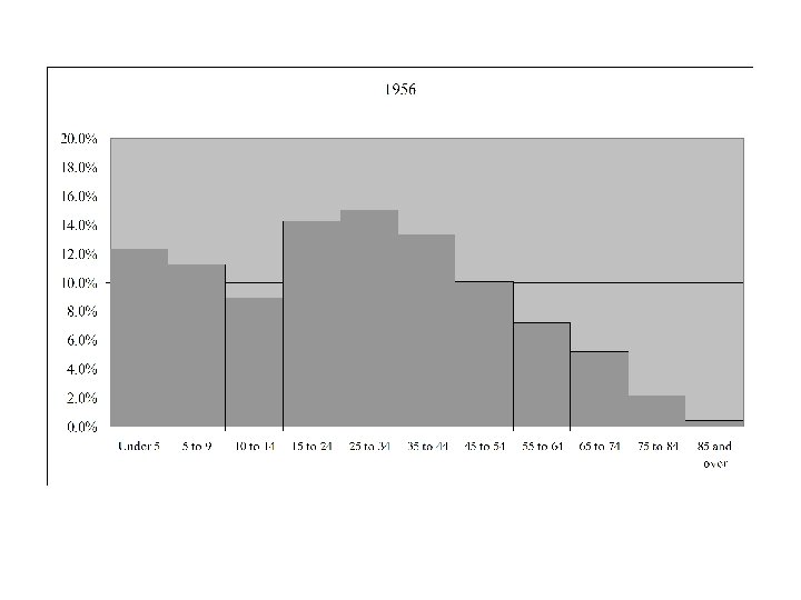
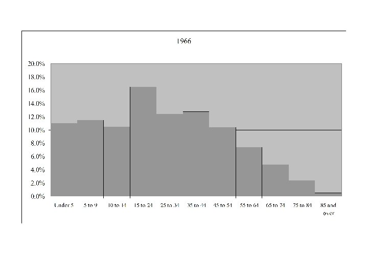
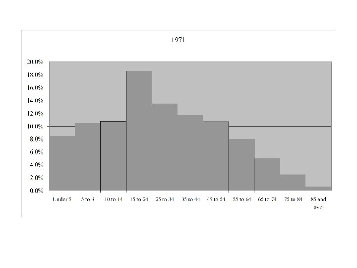
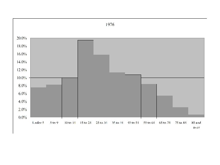
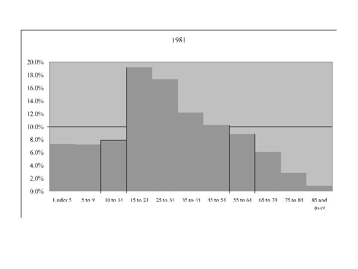
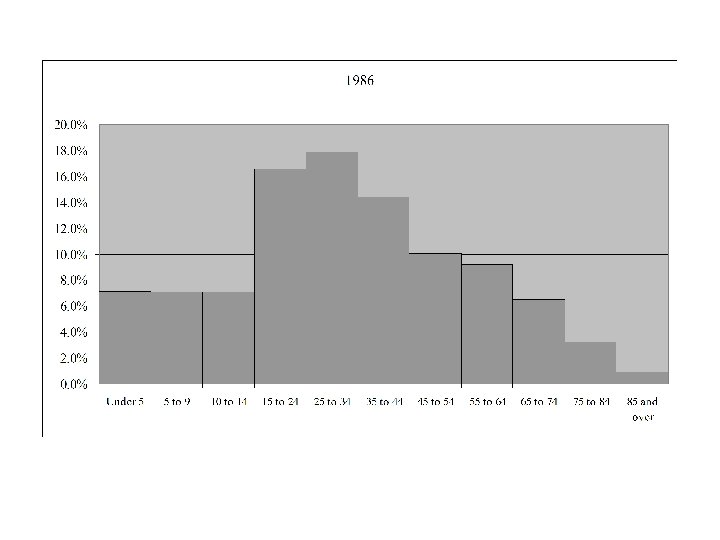
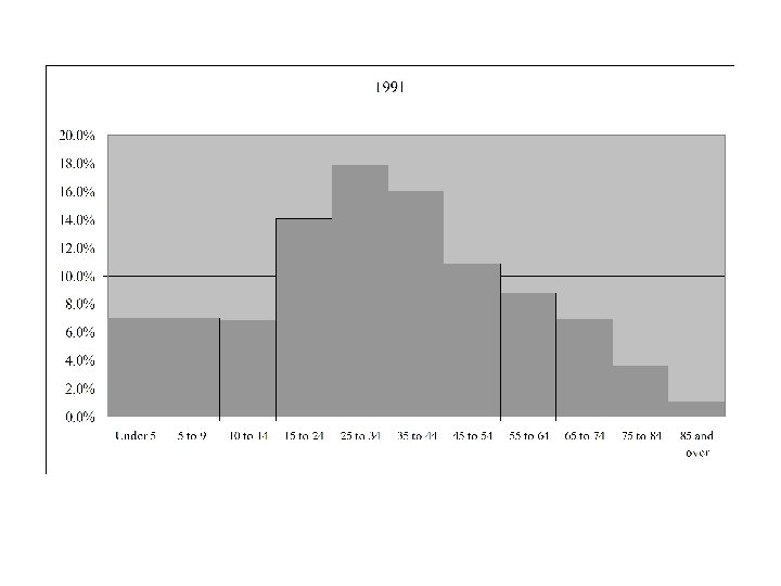
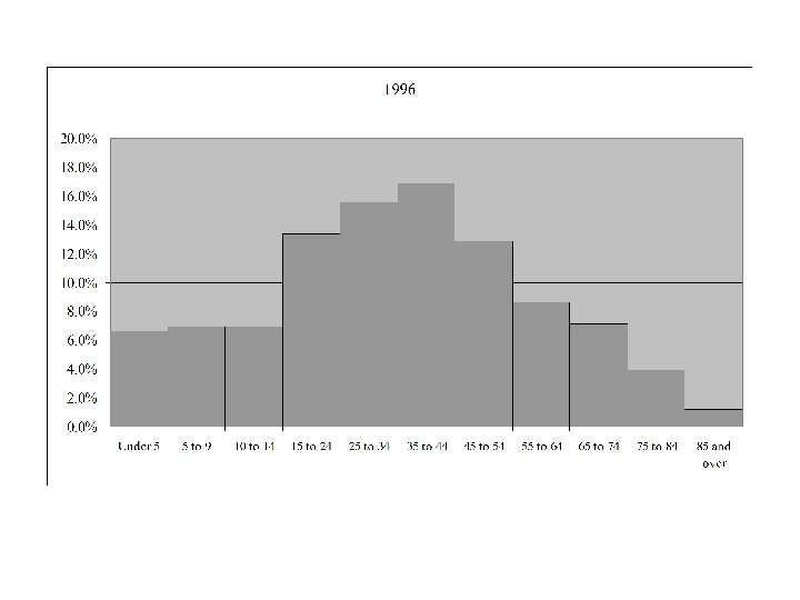
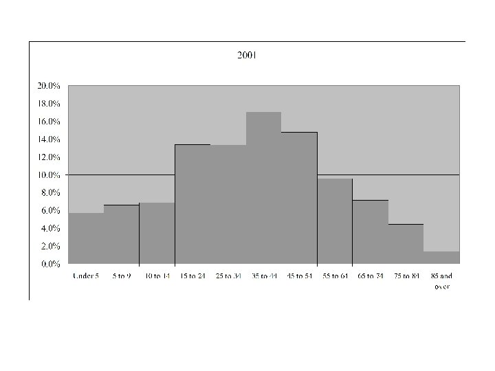
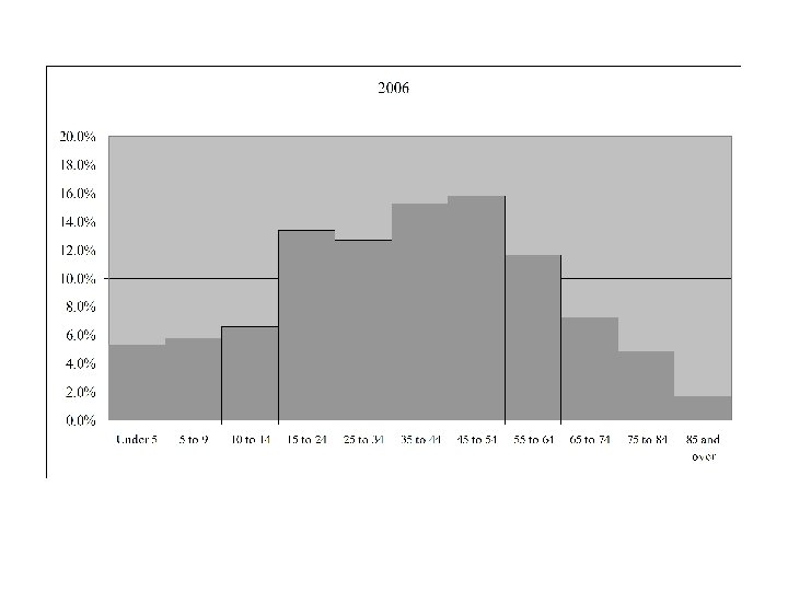
Example • The Baby Boom

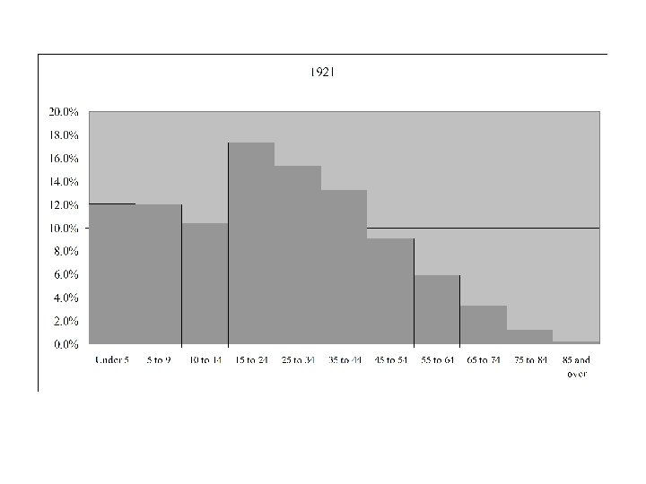
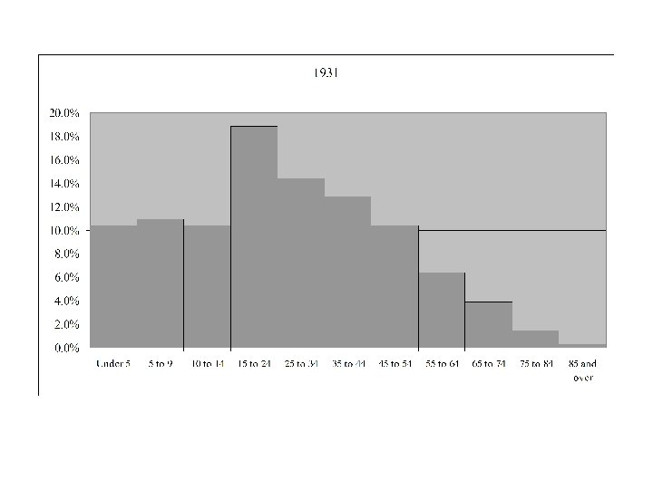
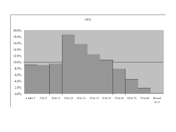
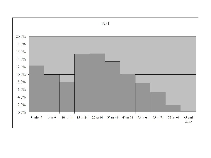
Age Distribution for Canada 1921 - 2006

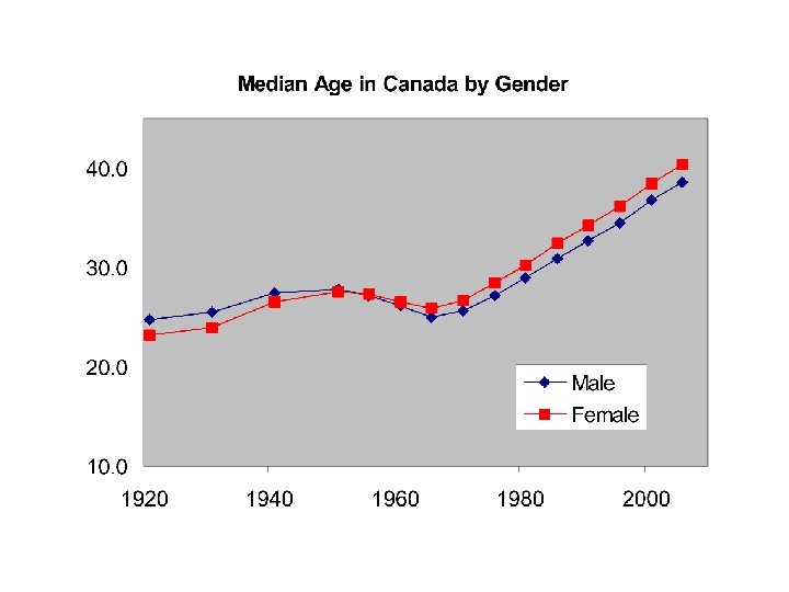
Median Age in Canada by Gender and Year

Total Population in Canada by Year

Summary Numerical Measures

Measure of Central Location 1. Mean 2. Median

Measure of Non-Central Location 1. Percentiles 2. Quartiles 1. Lower quartile (Q 1) (25 th percentile) (lower mid-hinge) 2. median (Q 2) (50 th percentile) (hinge) 3. Upper quartile (Q 3) (75 th percentile) (upper mid-hinge)

Measure of Variability (Dispersion, Spread) 1. 2. 3. 4. Range Inter-Quartile Range Variance, standard deviation Pseudo-standard deviation

1. Range R = Range = max - min 2. Inter-Quartile Range (IQR) Inter-Quartile Range = IQR = Q 3 - Q 1

Example The data Verbal IQ on n = 23 students arranged in increasing order is: 80 82 84 86 86 89 90 94 94 95 95 96 99 99 102 104 105 109 111 118 119 min = 80 Q 1 = 89 Q 2 = 96 Q 3 = 105 max = 119

Range and IQR Range = max – min = 119 – 80 = 39 Inter-Quartile Range = IQR = Q 3 - Q 1 = 105 – 89 = 16

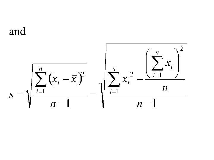
3. Sample Variance Let x 1, x 2, x 3, … xn denote a set of n numbers. Recall the mean of the n numbers is defined as:

The numbers are called deviations from the mean

The sum is called the sum of squares of deviations from the mean. Writing it out in full: or

The Sample Variance Is defined as the quantity: and is denoted by the symbol

The Sample Standard Deviation s Definition: The Sample Standard Deviation is defined by: Hence the Sample Standard Deviation, s, is the square root of the sample variance.

Interpretations of s • In Normal distributions – Approximately 2/3 of the observations will lie within one standard deviation of the mean – Approximately 95% of the observations lie within two standard deviations of the mean – In a histogram of the Normal distribution, the standard deviation is approximately the distance from the mode to the inflection point

Mode Inflection point s

2/3 s s

2 s

A Computing formula for sample variance: Sum of squares of deviations from the mean : The difficulty with this formula is that will have many decimals. The result will be that each term in the above sum will also have many decimals.

The sum of squares of deviations from the mean can also be computed using the following identity:

Then:

A quick (rough) calculation of s The reason for this is that approximately all (95%) of the observations are between and Thus

The Pseudo Standard Deviation (PSD) Definition: The Pseudo Standard Deviation (PSD) is defined by:

Properties • For Normal distributions the magnitude of the pseudo standard deviation (PSD) and the standard deviation (s) will be approximately the same value • For leptokurtic distributions the standard deviation (s) will be larger than the pseudo standard deviation (PSD) • For platykurtic distributions the standard deviation (s) will be smaller than the pseudo standard deviation (PSD)

Measures of Shape

Measures of Shape • Skewness • Kurtosis

• Skewness – based on the sum of cubes • Kurtosis – based on the sum of 4 th powers

The Measure of Skewness

The Measure of Kurtosis

Interpretations of Measures of Shape • Skewness g 1 > 0 g 1 = 0 g 1 < 0 • Kurtosis g 2 < 0 g 2 = 0 g 2 > 0

Advance Box Plots

• An outlier is a “wild” observation in the data • Outliers occur because – of errors (typographical and computational) – Extreme cases in the population • We will now consider the drawing of boxplots where outliers are identified

To Draw a Box Plot we need to: • Compute the Hinge (Median, Q 2) and the Mid-hinges (first & third quartiles – Q 1 and Q 3 ) • To identify outliers we will compute the inner and outer fences

The fences are like the fences at a prison. We expect the entire population to be within both sets of fences. If a member of the population is between the inner and outer fences it is a mild outlier. If a member of the population is outside of the outer fences it is an extreme outlier.

Inner fences

Lower inner fence f 1 = Q 1 - (1. 5)IQR Upper inner fence f 2 = Q 3 + (1. 5)IQR

Outer fences

Lower outer fence F 1 = Q 1 - (3)IQR Upper outer fence F 2 = Q 3 + (3)IQR

• Observations that are between the lower and upper inner fences are considered to be nonoutliers. • Observations that are outside the inner fences but not outside the outer fences are considered to be mild outliers. • Observations that are outside outer fences are considered to be extreme outliers.

• mild outliers are plotted individually in a box-plot using the symbol • extreme outliers are plotted individually in a box-plot using the symbol • non-outliers are represented with the box and whiskers with – Max = largest observation within the fences – Min = smallest observation within the fences

Box-Whisker plot representing the data that are not outliers Extreme outlier Mild outliers Inner fences Outer fence

Example Data collected on n = 109 countries in 1995. Data collected on k = 25 variables.

The variables 1. Population Size (in 1000 s) 2. Density = Number of people/Sq kilometer 3. Urban = percentage of population living in cities 4. Religion 5. lifeexpf = Average female life expectancy 6. lifeexpm = Average male life expectancy

7. literacy = % of population who read 8. pop_inc = % increase in popn size (1995) 9. babymort = Infant motality (deaths per 1000) 10. gdp_cap = Gross domestic product/capita 11. Region = Region or economic group 12. calories = Daily calorie intake. 13. aids = Number of aids cases 14. birth_rt = Birth rate per 1000 people

15. death_rt = death rate per 1000 people 16. aids_rt = Number of aids cases/100000 people 17. log_gdp = log 10(gdp_cap) 18. log_aidsr = log 10(aids_rt) 19. b_to_d =birth to death ratio 20. fertility = average number of children in family 21. log_pop = log 10(population)

22. cropgrow = ? ? 23. lit_male = % of males who can read 24. lit_fema = % of females who can read 25. Climate = predominant climate

The data file as it appears in SPSS

Consider the data on infant mortality Stem-Leaf diagram stem = 10 s, leaf = unit digit

Summary Statistics median = Q 2 = 27 Quartiles Lower quartile = Q 1 = the median of lower half Upper quartile = Q 3 = the median of upper half Interquartile range (IQR) IQR = Q 1 - Q 3 = 66. 5 – 12 = 54. 5

The Outer Fences lower = Q 1 - 3(IQR) = 12 – 3(54. 5) = - 151. 5 upper = Q 3 = 3(IQR) = 66. 5 + 3(54. 5) = 230. 0 No observations are outside of the outer fences The Inner Fences lower = Q 1 – 1. 5(IQR) = 12 – 1. 5(54. 5) = - 69. 75 upper = Q 3 = 1. 5(IQR) = 66. 5 + 1. 5(54. 5) = 148. 25 Only one observation (168 – Afghanistan) is outside of the inner fences – (mild outlier)

Box-Whisker Plot of Infant Mortality

Example 2 In this example we are looking at the weight gains (grams) for rats under six diets differing in level of protein (High or Low) and source of protein (Beef, Cereal, or Pork). – Ten test animals for each diet

Table Gains in weight (grams) for rats under six diets differing in level of protein (High or Low) and source of protein (Beef, Cereal, or Pork) High Protein Level Source Diet Median Mean IQR PSD Variance Std. Dev. Low protein Beef Cereal Pork 1 73 102 118 104 81 107 100 87 111 103. 0 100. 0 24. 0 17. 78 229. 11 15. 14 2 98 74 56 111 95 88 82 77 86 92 87. 0 85. 9 18. 0 13. 33 225. 66 15. 02 3 94 79 96 98 102 108 91 120 105 100. 0 99. 5 11. 0 8. 15 119. 17 10. 92 4 90 76 90 64 86 51 72 90 95 78 82. 0 79. 2 18. 0 13. 33 192. 84 13. 89 5 107 95 97 80 98 74 74 67 89 58 84. 5 83. 9 23. 0 17. 04 246. 77 15. 71 6 49 82 73 86 81 97 106 70 61 82 81. 5 78. 7 16. 0 11. 05 273. 79 16. 55

High Protein Beef Cereal Pork Low Protein Beef Cereal Pork

Conclusions • Weight gain is higher for the high protein meat diets • Increasing the level of protein - increases weight gain but only if source of protein is a meat source

Multivariate Data