Submodular Maximization in the Big Data Era Moran

Submodular Maximization in the Big Data Era Moran Feldman The Open University of Israel Based on • Greed Is Good: Near-Optimal Submodular Maximization via Greedy Optimization. Feldman, Harshaw and Karbasi. COLT 2017. • Do Less, Get More: Streaming Submodular Maximization with Subsampling. Feldman, Karbasi and Kazemi. NIPS 2018 (to appear). • Unconstrained Submodular Maximization with Constant Adaptive Complexity. Chen, Feldman and Karbasi. Submitted for publication.

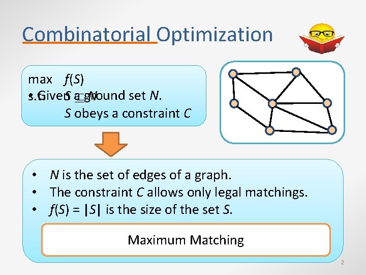
Combinatorial Optimization max f(S) • s. t. Given. S a ground set N. N S obeys a constraint C • N is the set of edges of a graph. • The constraint C allows only legal matchings. • f(S) = |S| is the size of the set S. Maximum Matching 2

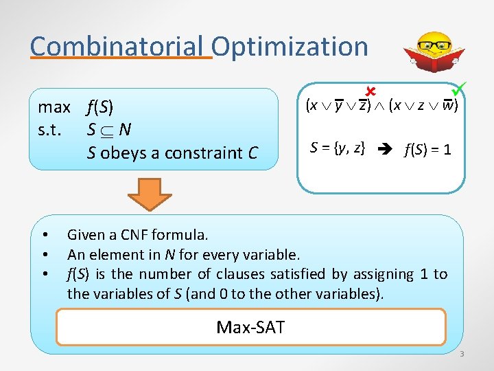
Combinatorial Optimization max f(S) s. t. S N S obeys a constraint C • • • (x y z) (x z w) S = {y, z} f(S) = 1 Given a CNF formula. An element in N for every variable. f(S) is the number of clauses satisfied by assigning 1 to the variables of S (and 0 to the other variables). Max-SAT 3

An Interesting Special Case max f(S) s. t. S N S obeys a constraint C • Generalizes Maximum Independent Set • Cannot be approximated • Interesting to study special cases. • Should have the right amount of structure. 4

An Interesting Special Case max f(S) s. t. S N S obeys a constraint C Well Known Example • The function f is linear. • C is defined by a totally unimodular matrix (a bit inaccurate). • Every element in N has a A matrix is totally unimodular weight. • Can be solved (exactly) efficiently. if the determinant of every Everysum extreme point solution integral. of it is either • f(S) is • the of the squareissubmatrix weights of S’s elements. -1, 0 or 1. 5

An Interesting Special Case max f(S) s. t. S N S obeys a constraint C In this Talk • Problems in which the objective function f is submodular. What is a submodular function? A class of functions capturing diminishing returns 6

Why should We Care? Diminishing returns (and thus, submodularity) appear everywhere. Economics Buying 100 apples is cheaper than buying them separately. Sensor Covering The more sensors there are, the less each one covers alone. 7

Why should We Care? Diminishing returns (and thus, submodularity) appear everywhere. Summarization Σ • Given a text, extract the a small set of sentences capturing most of the information. • Extract a small set of representative pictures from a video. Combinatorics For example, the cut function of a graph. 8

The Greedy Algorithm So, how do we maximize submodular functions? In practice, usually just run the greedy algorithm. The Greedy Algorithm 1. While more elements that can be added to the solution: 2. Pick among them the element increasing the value by the most. 3. Add it to the solution. 9

The Greedy Algorithm In 1978, proved to have a Intuitively works because theoretical approximation there are no synergies. guarantee in many cases. • If an element is good as part of Algorithm a group, then it is The Greedy [Fisher et al. , 1978] also more good elements alone. that can be added to the solution: 1. While 2. 3. [Nemhauser and Wolsey, 1978] Pick among them the element increasing the value by the most. [Nemhauser et al. , 1978] Add it to the solution. 10

More Recent History Research on submodular maximization boomed in the last decade. • Enabled by theoretical breakthroughs. • Motivated by many new applications, especially in machine learning. Better Guarantees • Better Approximations • More General Problems Doing it Faster • Less computation • Less objective evaluations Big Data Models • Streaming • Property Testing • Parallelism ‒ Map-Reduce ‒ Low Adaptivity 11

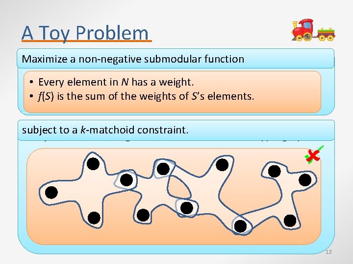
A Toy Problem Maximize submodular function Maximizeaanon-negative linear function • Every element in N has a weight. • f(S) is the sum of the weights of S’s elements. subject to a k-matchoid constraint. subject to a matching constraint in a k-uniform hypergraph. 12

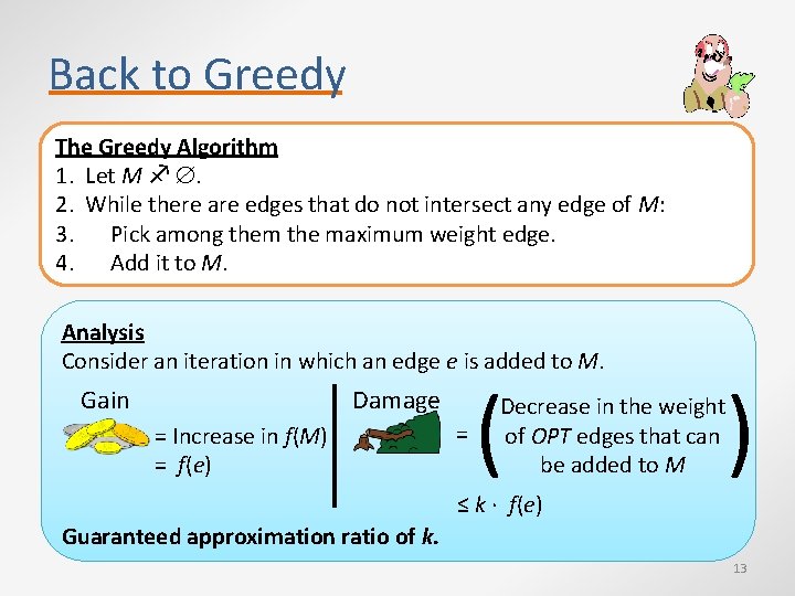
Back to Greedy The Greedy Algorithm 1. Let M . 2. While there are edges that do not intersect any edge of M: 3. Pick among them the maximum weight edge. 4. Add it to M. Analysis Consider an iteration in which an edge e is added to M. Gain Damage = Increase in f(M) = f(e) = ( Decrease in the weight of OPT edges that can be added to M ) ≤ k ∙ f(e) Guaranteed approximation ratio of k. 13

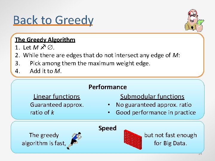
Back to Greedy The Greedy Algorithm 1. Let M . 2. While there are edges that do not intersect any edge of M: 3. Pick among them the maximum weight edge. 4. Add it to M. Linear functions Guaranteed approx. ratio of k The greedy algorithm is fast, Performance Submodular functions • No guaranteed approx. ratio • Good performance in practice Speed but not fast enough for Big Data. 14

Getting More Speed Previous work suggested implementations for the greedy algorithm that are faster either • in practice [Minoux, 1978], • or in theory [Badanidiyuru and Vondrák, 2014]. Can we gain speed by modifying the greedy algorithm? Sure, just remove a (random) part of the input. 15

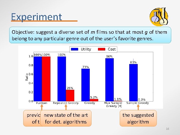
Experiment Objective: suggest a diverse set of m films so that at most g of them belong to any particular genre out of the user’s favorite genres. previousnew state of the art of thefor artdet. algorithms the suggested algorithm 16

Why does It Work? • Removing elements that do not belong to OPT is not a problem. • Removing elements of OPT is a problem only if greedy would have Results Take Home Message taken them otherwise. • No loss for linear functions. Removing random parts of • Now the algorithm has a the input makes sense when Reminder guaranteed approximation Balance ≤k accidently picking parts of When adding every element e: ratio for submodular OPT helps the algorithm. functions. - each = Increase in the value of the solution. = Decrease in the weight of OPT edges that can be other added to the solution. If e is an OPT element: =1 17

(Semi-)Streaming A computational model for the case in which the input is too large to store in memory. • Extracting from a long surveillance video a set of frames representing the “action” taking place. The edges of the hypergraph arrive one after the other. We only allowed memory linear in the size of the maximum possible solution (up to poly-logarithmic terms). 18

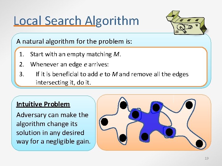
Local Search Algorithm A natural algorithm for the problem is: 1. Start with an empty matching M. 2. Whenever an edge e arrives: 3. If it is beneficial to add e to M and remove all the edges intersecting it, do it. Intuitive Problem Adversary can make the algorithm change its solution in any desired way for a negligible gain. 19

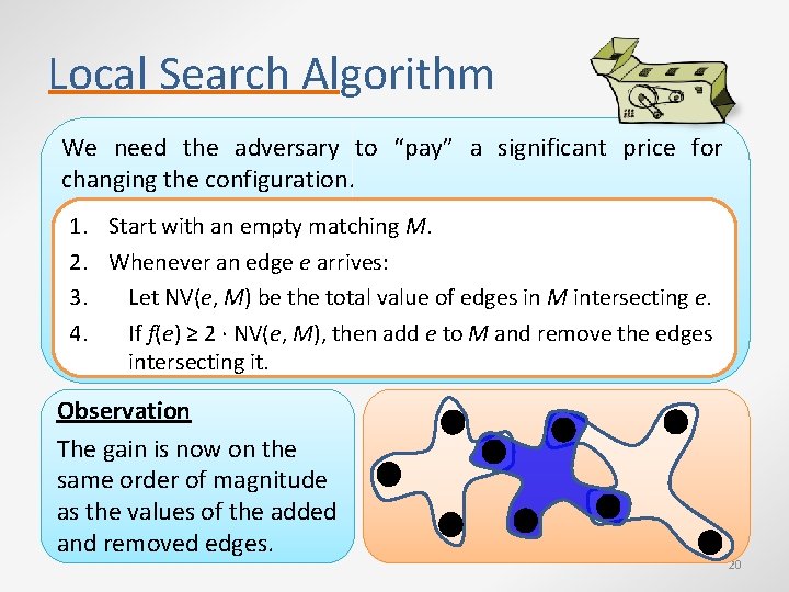
Local Search Algorithm We need the adversary to “pay” a significant price for changing the configuration. 1. Start with an empty matching M. 2. Whenever an edge e arrives: 3. Let NV(e, M) be the total value of edges in M intersecting e. 4. If f(e) ≥ 2 ∙ NV(e, M), then add e to M and remove the edges intersecting it. Observation The gain is now on the same order of magnitude as the values of the added and removed edges. 20

Our Contribution Linear functions • Guaranteed approx. ratio of 4 k [Chakrabarti and Kale (2014) and Chekuri et al. (2015)] • Improves when the algorithm takes many OPT elements Submodular functions No guaranteed approx. ratio • Same situation as with the greedy algorithm. • Natural to use the same “crazy” solution: Ø Ignore (at random) some of the arriving elements. • Faster algorithm. • No loss in the guarantee for linear functions. • Approximation guarantee for general submodular functions. 21

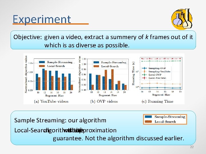
Experiment Objective: given a video, extract a summery of k frames out of it which is as diverse as possible. Sample Streaming: our algorithm Local-Search: algorithm with the state the art approximation of guarantee. Not the algorithm discussed earlier. 22

Adaptivity • • Algorithms for submodular maximization evaluate the objective function many times. In practice, these evaluations might be quite expensive. Obvious Conclusion • Try to reduce number of evaluations. • Usually equivalent to Think about the faster. making the alg. greedy algorithm… Other Option • Make the evaluations in parallel. • Problem: Most submodular optimization algorithms are inherently sequential. 23

Adaptivity Formal Model • • • The algorithm specifies the evaluations it wants in rounds (batches). Each round can include a polynomial number of evaluations. We want to keep the number of rounds small, so that the parallel execution time remains short. Some History Balkanski and Singer (2018) showed: • Algorithm for maximizing a monotone submodular function to subject to a cardinality constraint using O(log n) rounds. • Tight up to a O(log n) factor. • Many very recent extensions: general submodular functions, more general constraints. • All inherit the impossibility result. 24

Our Contribution Unconstrained submodular maximization Given a submodular function f, find a set maximizing it. Spoiler: Almost. . Optimal Approximation is 1/2 • Ignored by previous works. • Algorithm by Buchbinder et • An “ancient” algorithm • One can get (½ - ε)-approximation al. (2015). achieving 1/3 -approximation -1 using a singleusing roundÕ(ε of ) rounds. • Impossibility by Feige et al. We plan do experiments also. adaptivity. • [Feige et al. to 2011] (2011). Our Question Can one get the optimal ½-approximation using a constant number of rounds? 25

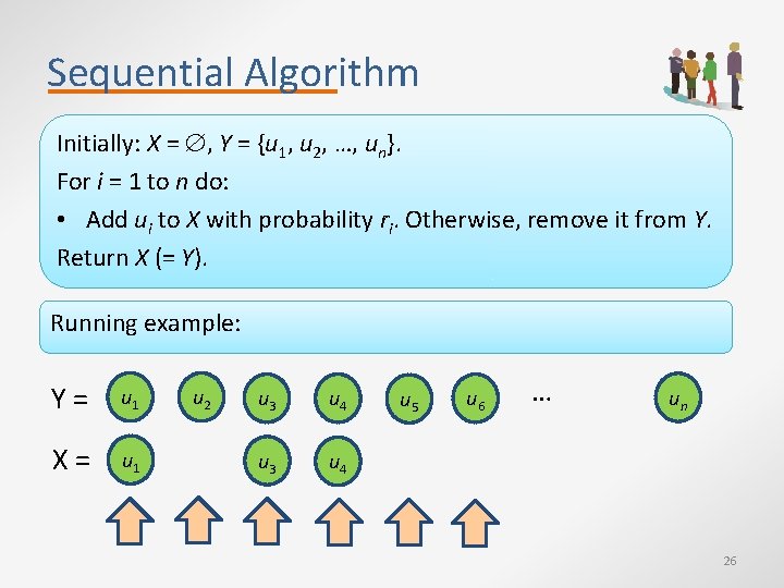
Sequential Algorithm Initially: X = , Y = {u 1, u 2, …, un}. For i = 1 to n do: • Add ui to X with probability ri. Otherwise, remove it from Y. Return X (= Y). Running example: Y= u 1 X= u 1 u 2 u 3 u 4 u 5 u 6 … un 26

Parallel Algorithm Goal • We want to make decisions for many of the elements in parallel. • Problem: the probability ri depends on the marginals of ui (how much one can gain by adding it to X or removing it from Y). Observation The marginals are more likely to change if we make decisions for more elements. There is a cutoff number. • The average marginal is likely to change for this number of decisions, • but not for fewer. 27

Cutoff • We make a decision for exactly this cutoff number of elements in every iteration. • Guarantees that every elements is chosen with (roughly) the right ri. How to find the cutoff? • Try an exponentially increasing series of values. • For every value, estimate by sampling. Bounding the number of rounds • The marginals can only decrease (diminishing returns). • After every round the average marginal is likely to decrease. • After a few rounds, the marginals are so low, allowing us to make all the remaining decisions in parallel. 28

Analysis of the Local Search Alg. Let S be the set maintained by the algorithm and A be the set of elements that have ever been in S. Observation 1 f(A) ≤ 2 ∙ f(S) Observation 2 f(OPT A) ≤ 2 k ∙ f(A OPT) Why? • The increase in f(S) is f(e) - NV(e, M) ≥ ½ ∙ f(e). • The increase in f(A) is f(e). 1. Start with an empty matching M. 2. Whenever an edge e arrives: 3. Let NV(e, M) be the total value of edges in M intersecting e. 4. If f(e) ≥ 2 ∙ NV(e, M), add e to M and remove edges intersecting it. 30

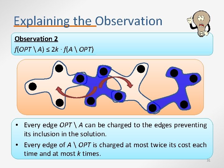
Explaining the Observation 2 f(OPT A) ≤ 2 k ∙ f(A OPT) • Every edge OPT A can be charged to the edges preventing its inclusion in the solution. • Every edge of A OPT is charged at most twice its cost each time and at most k times. 31

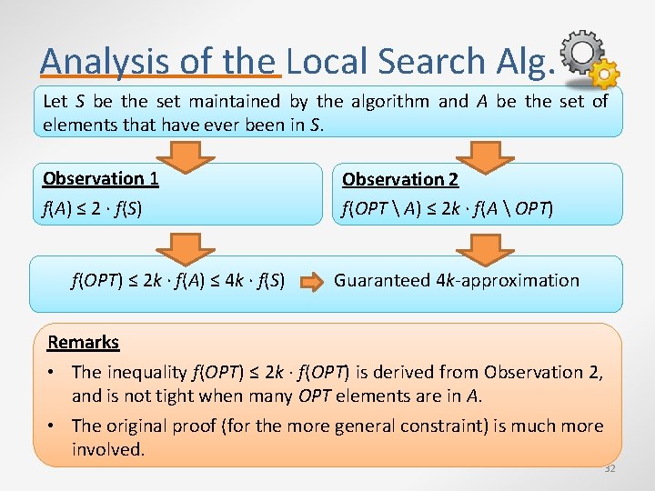
Analysis of the Local Search Alg. Let S be the set maintained by the algorithm and A be the set of elements that have ever been in S. Observation 1 f(A) ≤ 2 ∙ f(S) f(OPT) ≤ 2 k ∙ f(A) ≤ 4 k ∙ f(S) Observation 2 f(OPT A) ≤ 2 k ∙ f(A OPT) Guaranteed 4 k-approximation Remarks • The inequality f(OPT) ≤ 2 k ∙ f(OPT) is derived from Observation 2, and is not tight when many OPT elements are in A. • The original proof (for the more general constraint) is much more involved. 32