
Subjective Poverty and its Determinants an Empirical approach
Subjective Poverty and its Determinants: an Empirical approach to the Colombian case UNITED NATIONS ECONOMIC COMMISSION FOR EUROPE CONFERENCE OF EUROPEAN STATISTICIANS Seminar “Seminar on Poverty Measurement” (Geneva, 5 -6 May 2015) Luz Andrea Piñeros Ángela Bibiana González (Colombia)
Content 1. Motivation 2. Data and Methodology 4. Conclusions 3. Results 5. References
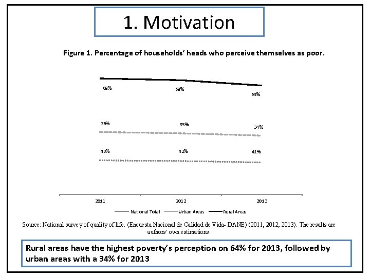
1. Motivation Figure 1. Percentage of households’ heads who perceive themselves as poor. 68% 36% 35% 43% 42% 2011 64% 34% 41% 2012 National Total Urban Areas 2013 Rural Areas Source: National survey of quality of life. (Encuesta Nacional de Calidad de Vida- DANE) (2011, 2012, 2013). The results are authors’ own estimations. Rural areas have the highest poverty’s perception on 64% for 2013, followed by urban areas with a 34% for 2013
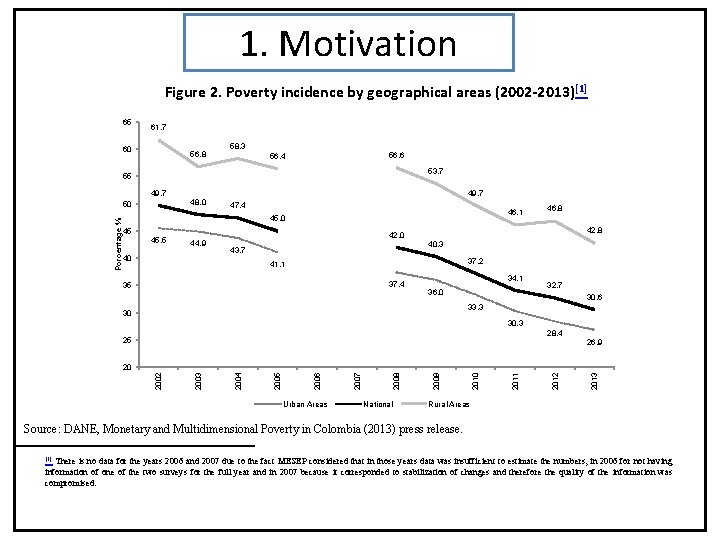
1. Motivation Figure 2. Poverty incidence by geographical areas (2002 -2013) [1] 65 61. 7 60 56. 8 58. 3 56. 6 56. 4 53. 7 55 49. 7 Porcentage % 49. 7 48. 0 50 47. 4 46. 1 45. 0 45 45. 5 44. 9 40 46. 8 42. 0 40. 3 43. 7 37. 2 41. 1 37. 4 35 34. 1 36. 0 32. 7 30. 6 33. 3 30 30. 3 28. 4 25 26. 9 Urban Areas National 2013 2012 2011 2010 2009 2008 2007 2006 2005 2004 2003 2002 20 Rural Areas Source: DANE, Monetary and Multidimensional Poverty in Colombia (2013) press release. There is no data for the years 2006 and 2007 due to the fact MESEP considered that in those years data was insufficient to estimate the numbers, in 2006 for not having information of one of the two surveys for the full year and in 2007 because it corresponded to stabilization of changes and therefore the quality of the information was compromised. [1]
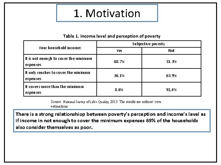
1. Motivation Table 1. Income level and perception of poverty Your household income: Subjective poverty Yes Not It is not enough to cover the minimum expenses 68. 7% 31. 3% It only reaches to cover the minimum expenses 36. 1% 63. 9% It covers more than the minimum expenses 8. 6% 91, 4% Source: National Survey of Life’s Quality, 2013. The results are authors’ own estimations. There is a strong relationshiop between poverty’s perception and income’s level as if income in not enough to cover the minimum expenses 69% of the households also consider themselves as poor.
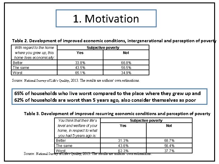
1. Motivation Table 2. Development of improved economic conditions, intergenerational and perception of poverty With regard to the home where you grew up, this home lives economically: Better The same Worst Subjective poverty Yes Not 33. 8% 43. 5% 65. 1% 66. 8% 56. 5% 34. 9% Source: National Survey of Life’s Quality, 2013. The results are authors’ own estimations. 65% of households who live worst compared to the place where they grew up and 62% of households are worst than 5 years ago, also consider themselves as poor Table 3. Development of improved recurring economic conditions and perception of poverty You think that their life’s Subjective poverty Yes Not level and welfare of your home, in respect to what you had 5 years ago is: Better 31. 3% 68. 7% The same 43. 6% 56. 4% Worst 62. 3% 37. 7% Source: National Survey of Life’s Quality, 2013. The results are authors’ own estimations.
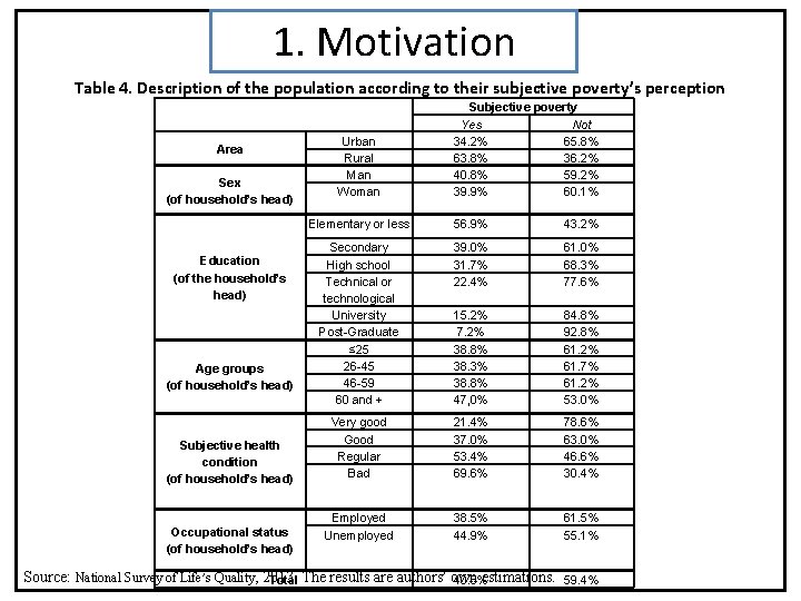
1. Motivation Table 4. Description of the population according to their subjective poverty’s perception Area Sex (of household’s head) Education (of the household’s head) Age groups (of household’s head) Subjective health condition (of household’s head) Occupational status (of household’s head) Urban Rural Man Woman Subjective poverty Yes Not 34. 2% 65. 8% 63. 8% 36. 2% 40. 8% 59. 2% 39. 9% 60. 1% Elementary or less 56. 9% 43. 2% Secondary High school Technical or technological University Post-Graduate ≤ 25 26 -45 46 -59 60 and + 39. 0% 31. 7% 22. 4% 61. 0% 68. 3% 77. 6% 15. 2% 7. 2% 38. 8% 38. 3% 38. 8% 47, 0% 84. 8% 92. 8% 61. 2% 61. 7% 61. 2% 53. 0% Very good Good Regular Bad 21. 4% 37. 0% 53. 4% 69. 6% 78. 6% 63. 0% 46. 6% 30. 4% Employed Unemployed 38. 5% 44. 9% 61. 5% 55. 1% Source: National Survey of Life’s Quality, 2013. estimations. Total The results are authors’ own 40. 6% 59. 4%
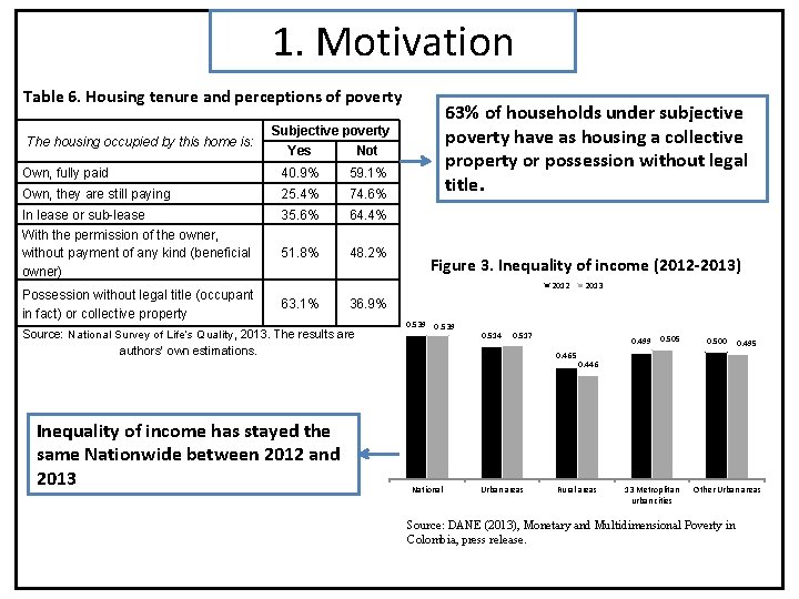
1. Motivation Table 6. Housing tenure and perceptions of poverty The housing occupied by this home is: Subjective poverty Yes Not Own, fully paid 40. 9% 59. 1% Own, they are still paying 25. 4% 74. 6% In lease or sub-lease With the permission of the owner, without payment of any kind (beneficial owner) 35. 6% 64. 4% 51. 8% 48. 2% Possession without legal title (occupant in fact) or collective property 63% of households under subjective poverty have as housing a collective property or possession without legal title. Figure 3. Inequality of income (2012 -2013) 2012 63. 1% 36. 9% Source: National Survey of Life’s Quality , 2013. The results are authors’ own estimations. Inequality of income has stayed the same Nationwide between 2012 and 2013 0. 539 0. 514 0. 517 0. 499 0. 465 National Urban areas 0. 505 0. 500 0. 495 0. 446 Rural areas 13 Metroplitan urban cities Other Urban areas Source: DANE (2013), Monetary and Multidimensional Poverty in Colombia, press release.
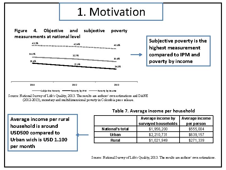
1. Motivation Figure 4. Objective and subjective measurements at national level 43. 2% 42. 4% 34. 1% poverty Subjective poverty is the highest measurement compared to IPM and poverty by income 40. 6% 32. 7% 30. 6% 29. 4% 27. 0% 2011 2012 Subjective Poverty by IPM 24. 8% 2013 Poverty by Income Source: National Survey of Life’s Quality, 2013. The results are authors’ own estimations and DANE (2012 -2013), monetary and multidimensional poverty in Colombia press release. Table 7. Average income per household Average income per rural household is around USD 500 compared to Urban wich is USD 1. 100 per month National’s total Urban Rural Average income by surveyed households $1, 956, 200 $2, 210, 731 $1, 021, 949 Average income person $555, 004 $639, 157 $271, 339 Source: National Survey of Life’s Quality, 2013. The results are authors’ own estimations.
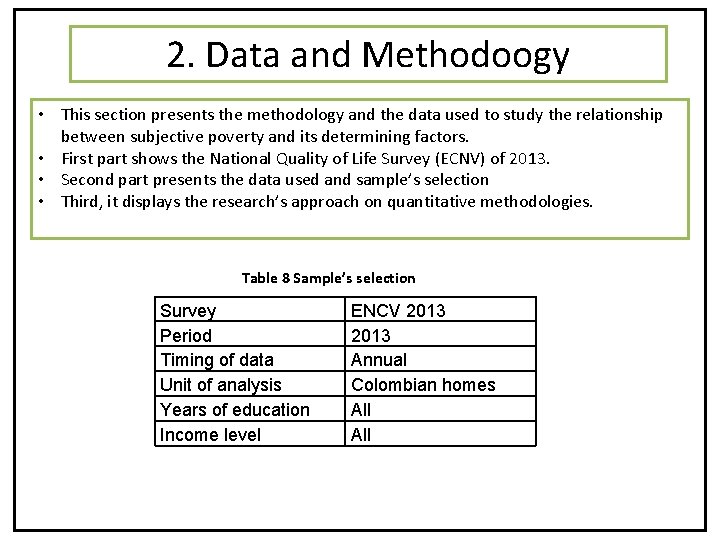
2. Data and Methodoogy • This section presents the methodology and the data used to study the relationship between subjective poverty and its determining factors. • First part shows the National Quality of Life Survey (ECNV) of 2013. • Second part presents the data used and sample’s selection • Third, it displays the research’s approach on quantitative methodologies. Table 8 Sample’s selection Survey Period Timing of data Unit of analysis Years of education Income level ENCV 2013 Annual Colombian homes All
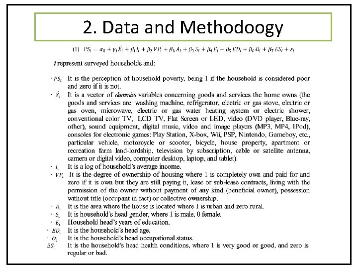
2. Data and Methodology 2. Data and Methodoogy
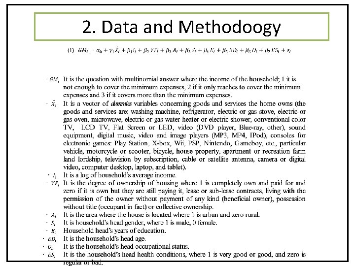
2. Data and Methodology 2. Data and Methodoogy
Dependent variable: subjective poverty Independent variables Clothes washing machine Fridge or refrigerator Gas or electric stove Electric or gas oven Microwave oven Electric water heater gas or electric shower Conventional colored TV Probit model (Marginal effects) -0. 193*** (0. 041) -0. 156*** (0. 032) -0. 060 (0. 056) -0. 188** (0. 054) -0. 026 (0. 061) -0. 304*** (0. 060) -0. 137** (0. 051) -0. 194*** TV LCD, Flat Screen or LED TV (0. 046) -0. 125*** Video player (DVD, Blue-ray, other) (0. 293) -0. 075** Sound equipment (0. 038) Digital music, video and image players (MP 3, -0. 104** Material assets MP 4, IPod) (0. 080) Consoles for electronic games: Play Station, -0. 019 (0. 079) X-box, Wii, PSP, Nintendo, Gameboy, etc. -0. 102*** Particular vehicle-car (0. 008) -0. 024 (0. 040) -0. 003 Bike (0. 038) Property on house, apartment or recreational -0. 119*** (0. 003) home 3. Results Homeownership Geographic area (0. 001) Gender of the head of household Education level of household’s head Motorcycle or scooter Television by subscription service, cable or satellite dish Digital / video camera Desktop computer Portable computer Tablet Income Average income per household (Log) -0. 141*** (0. 041) -0. 175** (0. 059) -0. 076 (0. 048) -0. 011 (0. 054) -0. 040 (0. 082) -0. 632*** (0. 102) 1 is own and fully paid and -0. 140*** (0. 004) zero the rest -0. 065*** 1 is urban and zero rural Years of household’s head 1 is male, 0 female 0. 125** (0. 043) Elementary or less 0. 500*** (0. 125) Secondary 0. 332** (0. 127) High school 0. 238*** (0. 012) Technical or technological -0. 165*** (0. 011) University -0. 115*** (0. 012) Post- Graduate -0. 349*** (0. 007) ≤ 25 -0. 120*** (0. 009) 26 -45 -0. 027*** (0. 001) 46 -59 -0. 111*** (0. 006) 60 and + 0. 213*** (0. 004) The household’s head Employee occupational status Household’s head health 1 is very good or good, condition and zero is regular or bad -0. 153*** (0. 008) -0. 268*** (0. 004)
Dependent variable: economic ladder Independent variables 1 -0. 189*** (0. 001) -0. 143*** (0. 003) -0. 229*** (0. 009) 0. 143 (0. 119) -0. 276*** (0. 001) -0. 687*** (0. 013) 2 -0. 116*** (0. 003) -0. 032*** (0. 000) -0. 112*** (0. 003) -0. 125*** (0. 002) -0. 132*** (0. 004) -0. 432*** (0. 011) 3 0. 210*** (0. 006) 0. 085*** (0. 001) 0. 485*** (0. 009) 0. 350*** (0. 007) 0. 227*** (0. 035) 0. 101*** (0. 002) -0. 073*** (0. 001) -0. 318*** (0. 008) -0. 094** (0. 001) -0. 127*** (0. 002) -0. 213*** (0. 003) -0. 101*** (0. 002) -0. 243 (0. 097) 0. 154*** (0. 006) 0. 146*** (0. 000) -0. 190*** (0. 002) Digital music, video and image -0. 175*** (0. 001) players (MP 3, MP 4, IPod) -0. 112*** (0. 001) -0. 127*** (0. 002) 0. 200*** (0. 005) 0. 409*** (0. 006) Consoles for electronic games: -0. 412*** Play Station, X-box, Wii, PSP, (0. 003) Nintendo, Gameboy, etc. -0. 199*** Particular vehicle-car -0. 345*** (0. 003) 0. 027*** (0. 001) -0. 117*** (0. 006) -0. 278*** (0. 008) 0. 234*** (0. 001) -0. 654*** (0. 018) 0. 493*** (0. 003) 0. 214** (0. 092) -0. 046 (0. 093) 0. 228*** (0. 003) -0. 189*** (0. 005) 0. 321*** (0. 002) -0. 119*** (0. 001) -0. 123*** (0. 004) -0. 105*** (0. 004) -0. 129*** (0. 005) 0. 542*** (0. 102) 0. 009 (0. 100) 0. 542*** (0. 100) 0. 121*** (0. 012) Clothes washing machine Fridge or refrigerator Gas or electric stove Electric or gas oven Microwave oven Electric water heater gas or electric shower Conventional color TV TV LCD, Flat screen or LED Video player (DVD, Blue-ray, other) Sound equipment Material assets (0. 002) -0. 325*** Motorcycle or scooter (0. 004) 0. 007 Bike (0. 084) Property on house, apartment -0. 325*** (0. 005) or recreational home -0. 078 Television by subscription service, cable or satellite dish (0. 080) -0. 126*** Digital / video camera Desktop computer Portable computer Tablet 3. Results Generalized ordered Logit Model (Marginal effects) (0. 005) -0. 038 (0. 106) -0. 168*** (0. 006) -0. 179*** (0. 001) Income Average income per household (Log) 1 is own and fully paid and zero the rest 1 is urban and zero rural -0. 765*** (0. 009) Homeownership -0. 248*** (0. 001) Geographic area -0. 189*** (0. 003) Gender of the head of 1 is male, 0 female -0. 167*** household (0. 004) Elementary or less 0. 431*** (0. 006) Secondary 0. 371*** (0. 001) High school 0. 302*** Education level of (0. 006) Technical or technological -0. 432*** household’s head (0. 003) University -0. 577*** (0. 002) Post- Graduate -0. 678*** (0. 008) ≤ 25 0. 193*** (0. 001) 26 -45 -0. 018*** (0. 000) Years of household’s 46 -59 -0. 331*** head (0. 002) 60 and + 0. 456*** (0. 004) The household’s head Employee -0. 238*** occupational status (0. 004) Household’s head health 1 is very good or good, and -0. 430*** condition zero is regular or bad (0. 007) -0. 687*** (0. 012) -0. 235*** (0. 009) -0. 346*** (0. 008) -0. 146*** (0. 007) 0. 456*** (0. 004) 0. 431*** (0. 002) -0. 318*** (0. 008) -0. 569*** (0. 002) -0. 653*** (0. 006) -0. 421*** (0. 007) 0. 083*** (0. 000) -0. 127*** (0. 003) -0. 225*** (0. 009) 0. 543*** (0. 001) 0. 579*** (0. 001) 0. 328*** (0. 005) 0. 776*** (0. 101) 0. 143*** (0. 087) 0. 275*** (0. 001) 0. 079*** (0. 000) -0. 156*** (0. 005) -0. 719*** (0. 012) -0. 476*** (0. 002) 0. 339*** (0. 018) 0. 789*** (0. 108) 0. 467*** (0. 088) 0. 042 (0. 243) 0. 229*** (0. 012) 0. 303*** (0. 015) -0. 451*** (0. 017) 0. 623*** (0. 013) 0. 429*** (0. 003)
3. Results Dependent variable: subjective poverty Independent variables 1 Income Present and previous living conditions Geographic area Average income per household (Log) Better The same Worse 1 is urban and zero rural Household’s head 1 is male, 0 female gender Elementary or less Secondary High school Household’s head level of education Technical technological University or Post-Graduate ≤ 25 26 -45 Household’s head age 46 -59 60 and + Household’s head Employee occupational status 1 is very good or good, 2 Probit model (Marginal effects) Socioeconomic level status 3 4 5 6 -0. 462*** (0. 013) -0. 416*** (0. 001) -0. 321*** (0. 027) -0. 231*** (0. 012) -0. 256*** (0. 041) -0. 214*** (0. 004) -0. 214*** (0. 012) 0. 165** (0. 098) 0. 316*** (0. 065) -0. 265*** (0. 001) 0. 123*** (0. 001) -0. 125*** (0. 001) 0. 187*** (0. 005) 0. 298*** (0. 012) -0. 145*** (0. 006) 0. 174*** (0. 004) -0. 114*** (0. 021) 0. 176*** (0. 013) 0. 341*** (0. 014) -0. 277*** (0. 009) 0. 221*** (0. 011) -0. 154*** (0. 008) 0. 111*** (0. 021) 0. 411*** (0. 001) -0. 268*** (0. 000) 0. 287*** (0. 007) -0. 219*** (0. 013) 0. 125*** (0. 032) 0. 371*** (0. 007) -0. 345*** (0. 018) 0. 342*** (0. 004) -0. 254*** (0. 017) 0. 165*** (0. 012) 0. 286*** (0. 001) -0. 276*** (0. 016) 0. 321*** (0. 003) 0. 114*** (0. 009) 0. 119*** (0. 012) 0. 118*** (0. 011) -0. 266*** (0. 021) 0. 109*** (0. 007) 0. 123*** (0. 009) 0. 223*** (0. 021) -0. 135*** (0. 020) 0. 156*** (0. 002) 0. 187*** (0. 015) 0. 175*** (0. 041) -0. 204*** (0. 001) 0. 287*** (0. 019) 0. 225*** (0. 021) 0. 116*** (0. 016) -0. 198*** (0. 004) 0. 376*** (0. 021) 0. 265*** (0. 031) 0. 315*** (0. 009) -0. 231*** (0. 009) 0. 381*** (0. 028) 0. 314*** (0. 011) 0. 265*** (0. 081) -0. 567*** (0. 089) -0. 211*** (0. 006) -0. 462*** (0. 072) 0. 108*** (0. 012) -0. 154*** (0. 021) -0. 286*** (0. 012) 0. 176*** (0. 021) -0. 345*** (0. 032) -0. 226*** (0. 011) -0. 315*** (0. 021) 0. 121*** (0. 031) -0. 186*** (0. 018) -0. 172*** (0. 023) 0. 154*** (0. 032) -0. 281*** (0. 017) -0. 295*** (0. 024) -0. 262*** (0. 017) 0. 157*** (0. 009) -0. 116*** (0. 015) -0. 189*** (0. 019) 0. 152*** (0. 012) -0. 121*** (0. 014) -0. 219*** (0. 081) -0. 212*** (0. 011) 0. 114*** (0. 035) -0. 163*** (0. 013) -0. 103*** (0. 021) 0. 132*** (0. 021) -0. 367*** (0. 013) -0. 177*** (0. 016) -0. 198*** (0. 008) 0. 227*** (0. 042) -0. 125*** (0. 027) -0. 115*** (0. 023) 0. 118*** (0. 013) -0. 371*** (0. 005) -0. 354*** (0. 061) -0. 116*** (0. 005) 0. 098*** (0. 001) -0. 119*** (0. 006) -0. 214*** (0. 002) 0. 121*** (0. 009) -0. 289*** (0. 026) -0. 163*** -0. 131*** -0. 126*** -0. 312*** -0. 252*** -0. 235***
4. Conclusions • Usually most studies may not capture the subjective dimension of poverty and welfarethey consider income as relevant variable, but ignore other ones which affect the welfare’s level of the population under study. • This document proposes to study the subjective poverty and additionally, compares this measurement with objective indicators of material welfare and social capital; highlighting inequality’s perception as a fundamental factor to explain the high proportion of household’s head or spouses who feel poor. • Subjective poverty is defined by the people who respond they consider themselves as poor or also respond to the question of income on an economic scale. • Any attempt to define and measure poverty implies a judgmental assessment, about what constitutes good or bad living conditions. • This document examines subjective poverty since it considers studying individual’s selfperception is less imperfect and helps to form a more comprehensive judgment. • Little is known in Colombia about households’ perception of welfare. Thus, some households classified as not poor according to the criteria of expenditure or their income (objective measurements), may feel poor. Similarly, families who are considered poor by objective monetary indicators, they can perceive themselves as non-poor.
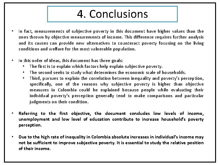
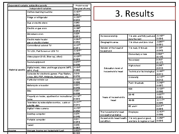
4. Conclusions • In fact, measurements of subjective poverty in this document have higher values than the ones thrown by objective measurements of income. This difference requires further analysis and its causes can provide new alternatives to counteract poverty focusing on the living conditions and welfare for the most vulnerable population. • In this order of ideas, this document has three goals: • The first is to explain which factors help explain subjective poverty. • The second seeks to study what determines the economic scale of households. • Third, pursues to explain the correlation between inequality and poverty’s perception, specifically, one of the reasons why subjective poverty is higher than objective measures in Colombia could be explained because people while evaluating their individual poverty’s perception generally tend to make comparisons and particular judgments on their condition. • Referring to the first objective, the document concludes low levels of income, unemployment and low level of education contribute to increase household’s poverty perception. • Due to the high rate of inequality in Colombia absolute increases in individual’s income may not be sufficient to improve subjective poverty. It is essential to study the relative position of their income.
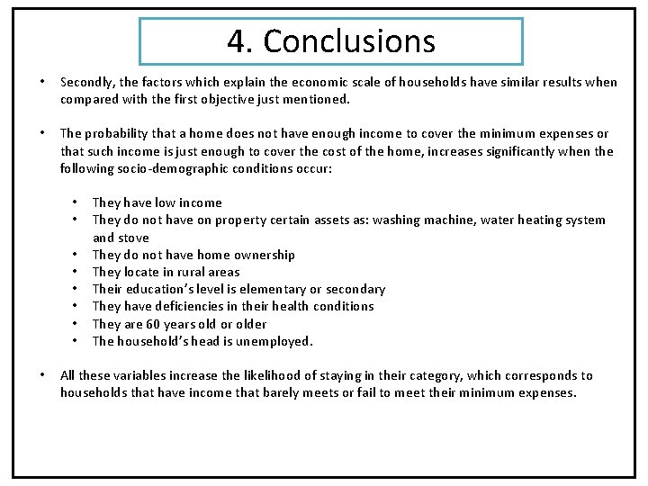
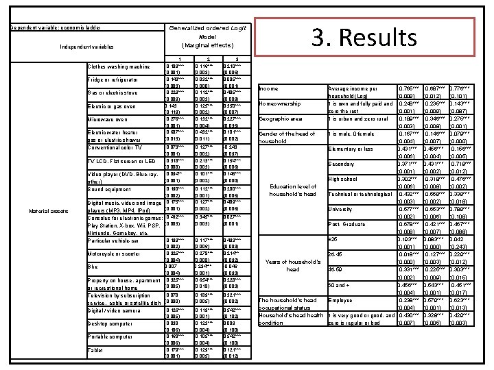
4. Conclusions • Secondly, the factors which explain the economic scale of households have similar results when compared with the first objective just mentioned. • The probability that a home does not have enough income to cover the minimum expenses or that such income is just enough to cover the cost of the home, increases significantly when the following socio-demographic conditions occur: • • • They have low income They do not have on property certain assets as: washing machine, water heating system and stove They do not have home ownership They locate in rural areas Their education’s level is elementary or secondary They have deficiencies in their health conditions They are 60 years old or older The household’s head is unemployed. All these variables increase the likelihood of staying in their category, which corresponds to households that have income that barely meets or fail to meet their minimum expenses.
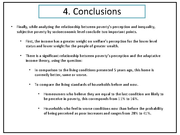
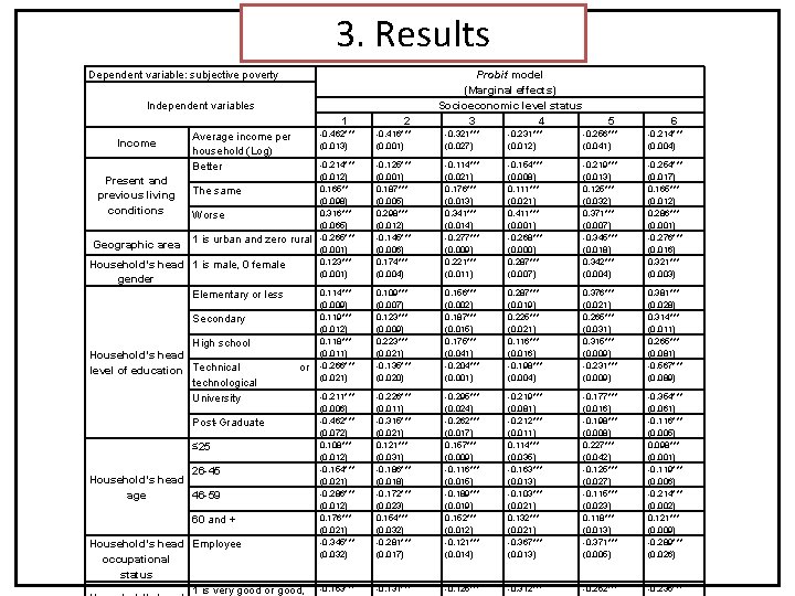
4. Conclusions • Finally, while analyzing the relationship between poverty’s perception and inequality, subjective poverty by socioeconomic level conclude two important points. • • First, the income has a greater weight on welfare’s perception for the lower level status and lower weight for the people of greater wealth. There is a significant relationship between poverty’s perception and the adaptative income theory, using the question: • In comparison to the living conditions presented 5 years ago, this home is currently better, same or worse. • To compare the living standards of households before and now. • Homeowners who believe they are equal to the last condition are likely to be perceive in poverty, this corresponds from 11% to 16%. • Households who feel in worse conditions now than before the probability of being perceived as poor increases and ranges from 28% to 41%.
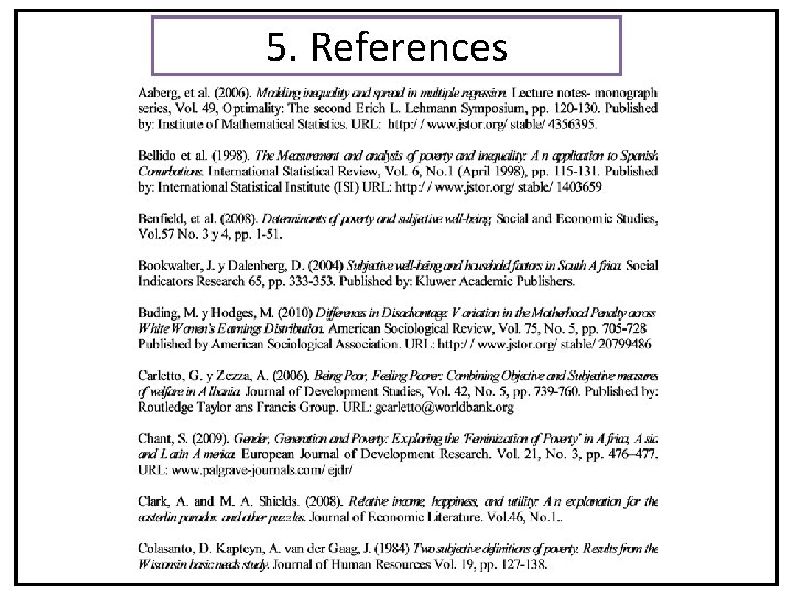
5. References
5. References
5. References
5. References
Many thanks!
- Slides: 24