Subject Outlines Subject title Data Structures Text book

Subject Outlines: Subject title : Data Structures • Text book: An Introduction To Data Structures With Application By Tremblay, J. P. , P. G. Sorenson. Second Edition. • Ref. book: Data Structures Using C and C++ By Langsam, Augenstein, Tenenbaum Teaching Scheme: Theory : 4 Lectures/week Practical: 4 hrs / Batch/week Examination Scheme: External theory : 60 Marks , Internal Exam: 40 Marks = 100 Practical + Termwork : 50 (25+25) Total=150 Marks 1

Data Structure • a data structure is a particular way of storing and organizing data so that it can be used efficiently. • Data structure usually consists of two things: • The type of structure that we are going to use to store data and how efficiently we perform operations onto that data stored in structure so that it results in less execution time and memory space require. • Different kinds of data structures are suited to different kinds of applications For example : • An array data structure stores a number of elements of the same type in a specific order. Arrays may be fixed-length or expandable. • Record : Records are among the simplest data structures. A record is a value that contains other values, typically in fixed number and sequence and typically indexed by names. 2

Data Structure describes, • how to store a collection of objects in memory, • what operations we can perform on that data, • the algorithms for those operations, and • how time and space efficient those algorithms are. q. A logical relationship among data elements that support specific data manipulation functions. q. Some data structures are linear in fashion. some are nonlinear. q. In linear data structure processing of data items is done in linear fashion. Linear adjacency is exist among the data. 3

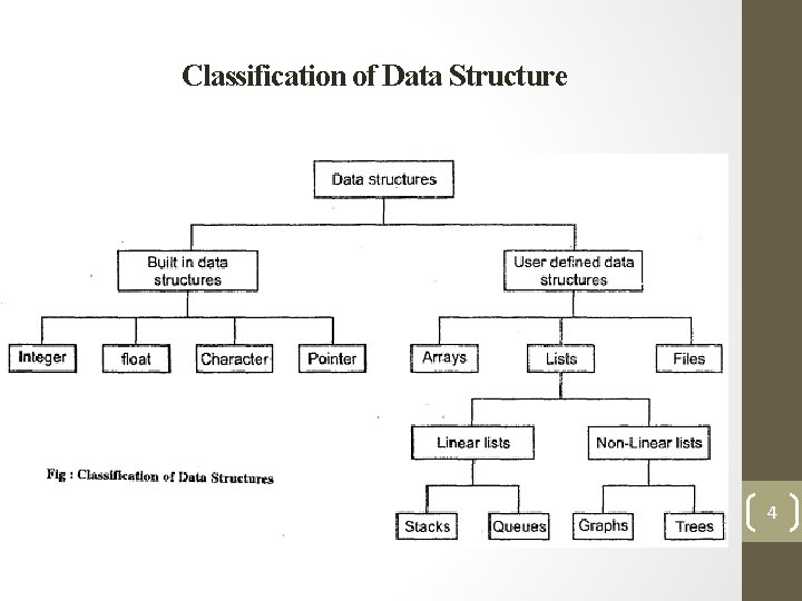
Classification of Data Structure 4

Difference Between Primitive and Non Primitive Data Structure • Primitive data structure: • These are data structures that can be manipulated directly by machine instructions. • In C language, the different primitive data structures are int, float, char, double. • Primitive data are only single values, they have not special capabilities. • Non primitive data structures: • These are data structures that can not be manipulated directly by machine instructions. Arrays, linked lists, files etc. , are some of non-primitive data structures and are classified into linear data structures and non-linear data structures. • The non-primitive data types are used to store the group of values. 5

Difference Between linear and Non linear Data Structure Linear data structure: • In linear data structures, data elements are organized sequentially and therefore they are easy to implement in the computer’s memory. • Some commonly used linear data structures are arrays, linked lists, stacks and queues. Non-linear data structure: • In nonlinear data structures, data elements are not organized in a sequential fashion. • they might be difficult to be implemented in computer’s linear memory. • Trees, graphs and files are non-linear data structures. 6

Definition of Algorithm • An algorithm is a sequence of finite number of steps to solve a specific problem. • A algorithm can be defined as well –defined step by step computational procedure which takes set of values as input and produce set of values as output. • A finite set of instruction that followed to accomplish a particular task. 7

Algorithm Terminology : format conventions 1. Name of algorithm: every algorithm is given an identifying name. the name written in capital letter. 2. Introductory comments: the algorithms name is followed by a brief introduction regarding the task the algorithm will perform. in addition it also discuss some assumptions. For example: SUM(A, N): this algorithm find the sum of all N elements in vector A. N is integer type variable indicate there are N elements in Vector A. 8

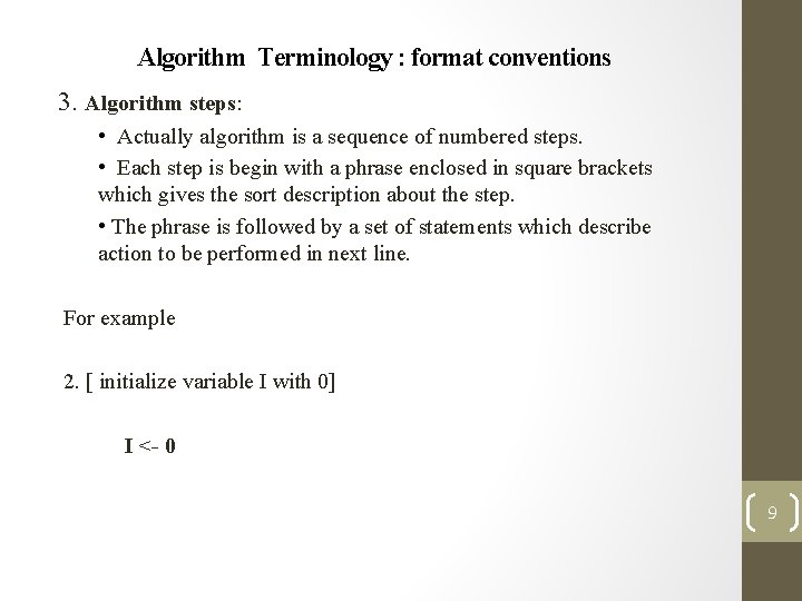
Algorithm Terminology : format conventions 3. Algorithm steps: • Actually algorithm is a sequence of numbered steps. • Each step is begin with a phrase enclosed in square brackets which gives the sort description about the step. • The phrase is followed by a set of statements which describe action to be performed in next line. For example 2. [ initialize variable I with 0] I <- 0 9

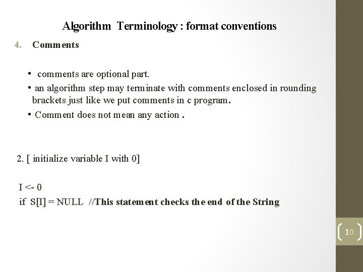
Algorithm Terminology : format conventions 4. Comments • comments are optional part. • an algorithm step may terminate with comments enclosed in rounding brackets just like we put comments in c program. • Comment does not mean any action. 2. [ initialize variable I with 0] I <- 0 if S[I] = NULL //This statement checks the end of the String 10

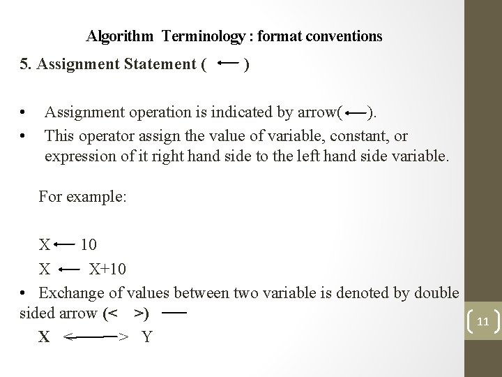
Algorithm Terminology : format conventions 5. Assignment Statement ( • • ) Assignment operation is indicated by arrow( ). This operator assign the value of variable, constant, or expression of it right hand side to the left hand side variable. For example: X 10 X X+10 • Exchange of values between two variable is denoted by double sided arrow (< >) X < > Y 11

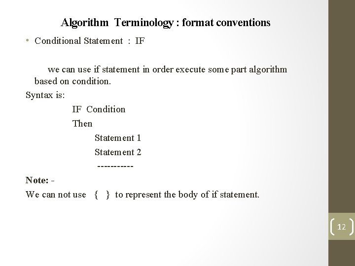
Algorithm Terminology : format conventions • Conditional Statement : IF we can use if statement in order execute some part algorithm based on condition. Syntax is: IF Condition Then Statement 1 Statement 2 -----Note: We can not use { } to represent the body of if statement. 12

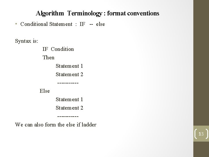
Algorithm Terminology : format conventions • Conditional Statement : IF -- else Syntax is: IF Condition Then Statement 1 Statement 2 -----Else Statement 1 Statement 2 -----We can also form the else if ladder 13

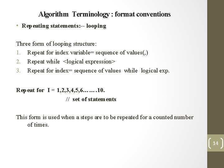
Algorithm Terminology : format conventions • Repeating statements: -- looping Three form of looping structure: 1. Repeat for index variable= sequence of values(, ) 2. Repeat while <logical expression> 3. Repeat for index= sequence of values while logical exp. Repeat for I = 1, 2, 3, 4, 5, 6……. 10. // set of statements This form is used when a steps are to be repeated for a counted number of times. 14

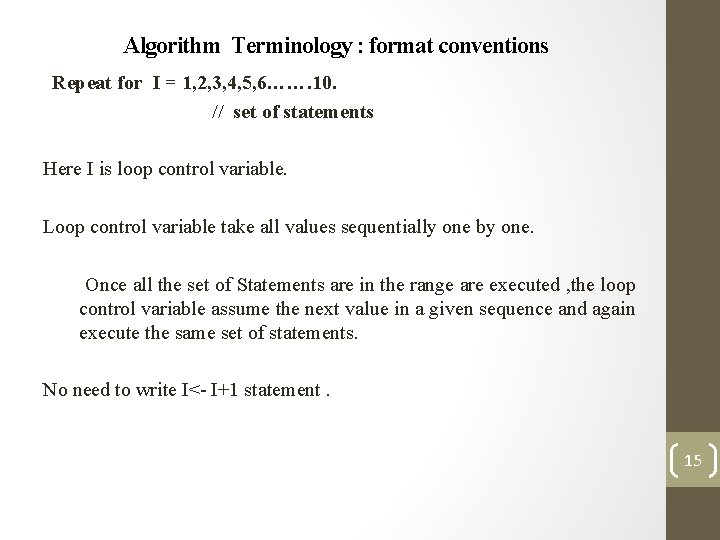
Algorithm Terminology : format conventions Repeat for I = 1, 2, 3, 4, 5, 6……. 10. // set of statements Here I is loop control variable. Loop control variable take all values sequentially one by one. Once all the set of Statements are in the range are executed , the loop control variable assume the next value in a given sequence and again execute the same set of statements. No need to write I<- I+1 statement. 15

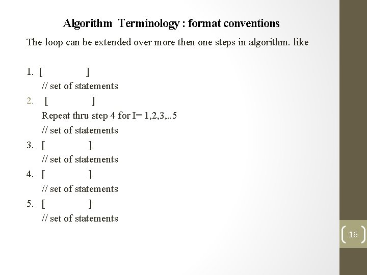
Algorithm Terminology : format conventions The loop can be extended over more then one steps in algorithm. like 1. [ ] // set of statements 2. [ ] Repeat thru step 4 for I= 1, 2, 3, . . 5 // set of statements 3. [ ] // set of statements 4. [ ] // set of statements 5. [ ] // set of statements 16

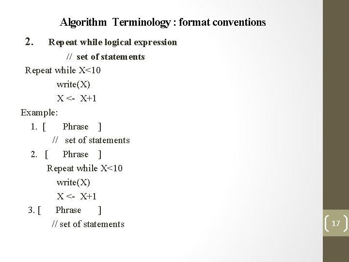
Algorithm Terminology : format conventions 2. Repeat while logical expression // set of statements Repeat while X<10 write(X) X <- X+1 Example: 1. [ Phrase ] // set of statements 2. [ Phrase ] Repeat while X<10 write(X) X <- X+1 3. [ Phrase ] // set of statements 17

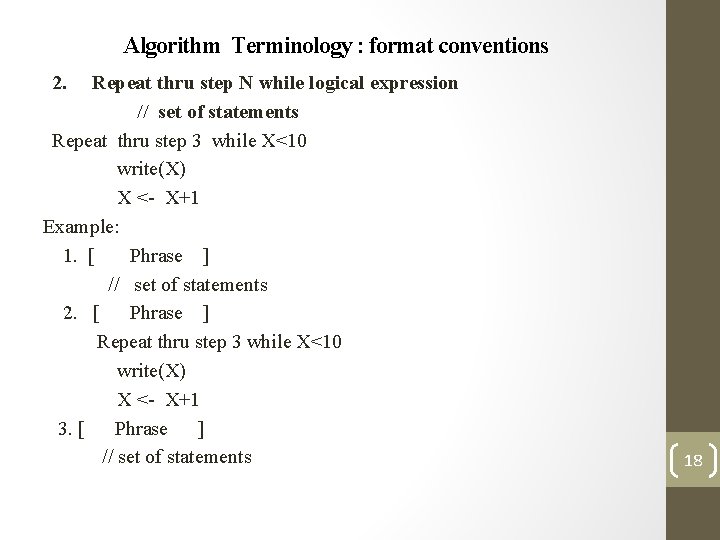
Algorithm Terminology : format conventions 2. Repeat thru step N while logical expression // set of statements Repeat thru step 3 while X<10 write(X) X <- X+1 Example: 1. [ Phrase ] // set of statements 2. [ Phrase ] Repeat thru step 3 while X<10 write(X) X <- X+1 3. [ Phrase ] // set of statements 18

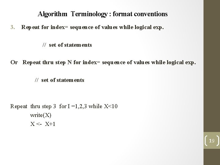
Algorithm Terminology : format conventions 3. Repeat for index= sequence of values while logical exp. // set of statements Or Repeat thru step N for index= sequence of values while logical exp. // set of statements Repeat thru step 3 for I =1, 2, 3 while X<10 write(X) X <- X+1 19

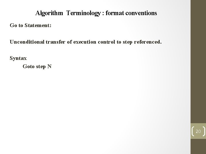
Algorithm Terminology : format conventions Go to Statement: Unconditional transfer of execution control to step referenced. Syntax Goto step N 20

QUEUE Data Structure • A Queue is a special kind of data structure in which elements are added at one end (called the rear), and elements are removed from the other end (called the front). • You come across a number of examples of a queue in real life situations. • For example, consider a line of students at a fee counter. Whenever a student enters the queue, he stands at the end of the queue. • Every time the student at the front of the queue deposits the fee, he leaves the queue. • The student who comes first in the queue is the one who leaves the queue first. • Since the first item inserted is the first item removed, a queue is commonly called a first-in-first-out or a FIFO data structure. 21

QUEUE Data Structure 8 Closely related to Stacks 8 It is a linear Data Structure 8 Queues are a first in first out data structure – FIFO 8 Add items to the end of the queue 8 Access and remove from the front 8 Used extensively in operating systems – Queues of processes, I/O requests, and much more 22

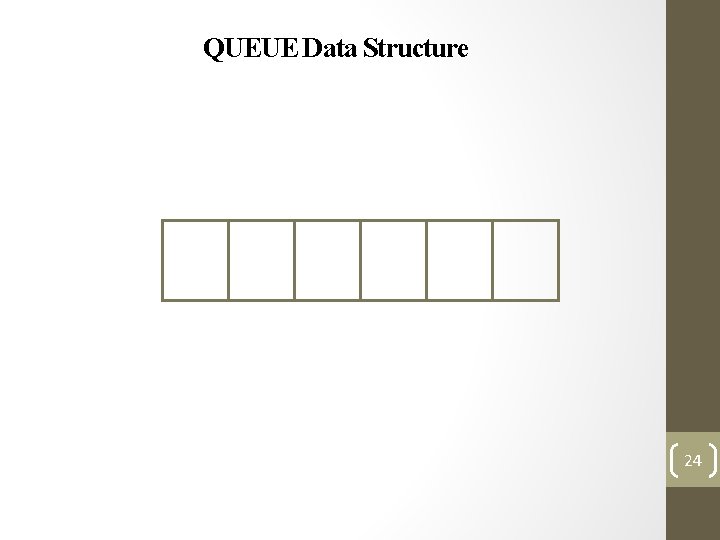
QUEUE Data Structure How do we keep track which element to be removed and where the new element to be added to queue? ? ? ? We require to maintain Two pointer in order to perform the insertion and deletion operations in queue. The Rear pointer is used to insert an elements in a queue. The Front pointer is used to delete an elements from the queue. Array Implementation of QUEUE: 1. Array Declaration 2. Front pointer 3. Rear Pointer 23

QUEUE Data Structure 24

Basic Queue Operations n Creating and Initializing the Queue. n Inserting an element into Queue. n Deleting an element from the Queue. n Is the Queue empty? n Is the Queue full? 25

Creating Queue • There are Two way to implement the Queue Data structure • • Static Implementation of queue Dynamic Creation of queue. • The first approach is implementing Queue using ARRAY. • The Second approach is implementing Queue using Linked List(pointer). 26

Array Implementation of Queue Array implementation of queue require followings: • Declare an array of appropriate size. • Create two index variable which will work as a front and rear of the queue. • During queue operations queue may grow or shrink within the space reserved for it. • When queue is empty , front and rear variable has value -1. when queue has one element , front and rear variable has value 0, when queue has 2 elements then front variable has value 0 and rear variable has value 1 , so on called queue is growing. 27

Array Implementation of Queue • When queue has Size-1 elements then we can say queue is full. Next insert operation put the queue in overflow condition. • In short, every insert operation increment the value of rear variable by 1. • Similarly every delete operation remove front element from the queue and increment the front variable by 1. • When front and rear variable point to the same position means queue is empty and both initialization with -1. 28

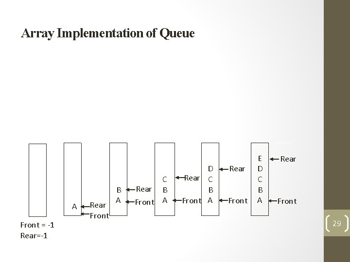
Array Implementation of Queue A Front = -1 Rear=-1 Rear Front B A C Rear B Front A D Rear C B Front A Rear Front E D C B A Rear Front 29

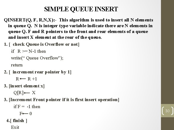
SIMPLE QUEUE INSERT QINSERT(Q, F, R, N, X): - This algorithm is used to insert all N elements in queue Q. N is integer type variable indicate there are N elements in queue Q. F and R pointers to the front and rear elements of a queue and insert X element at the rear of the queue. 1. [ check Queue is Overflow or not] if R >= N-1 then write(“ Queue Overflow”); return 2. [ increment rear pointer by 1] R R +1 3. [insert element x] Q[R] X 3. [Increment Front pointer if it is first insert operation] if F = -1 then F 0 4. [ finish ] Exit 30

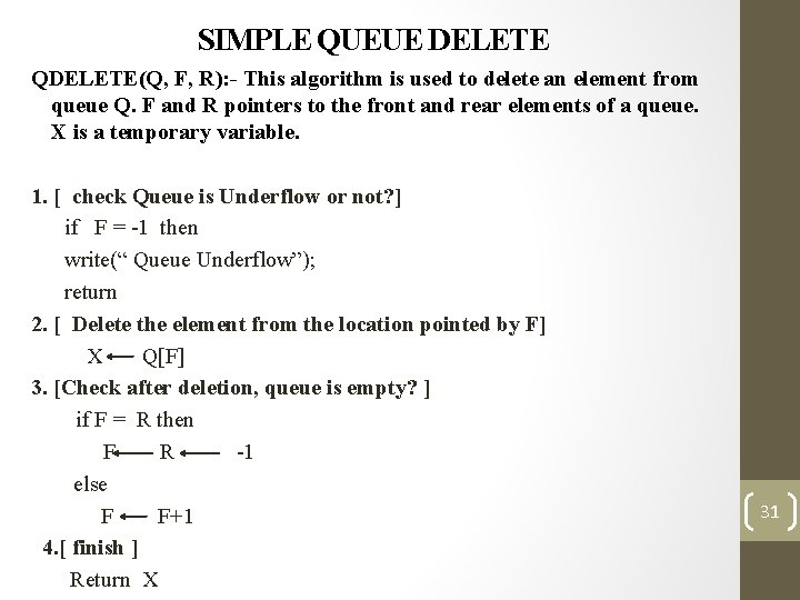
SIMPLE QUEUE DELETE QDELETE(Q, F, R): - This algorithm is used to delete an element from queue Q. F and R pointers to the front and rear elements of a queue. X is a temporary variable. 1. [ check Queue is Underflow or not? ] if F = -1 then write(“ Queue Underflow”); return 2. [ Delete the element from the location pointed by F] X Q[F] 3. [Check after deletion, queue is empty? ] if F = R then F R -1 else F F+1 4. [ finish ] Return X 31

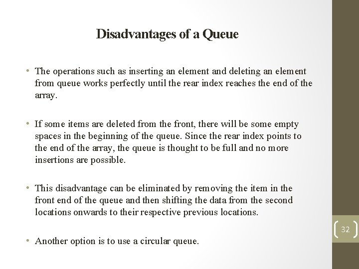
Disadvantages of a Queue • The operations such as inserting an element and deleting an element from queue works perfectly until the rear index reaches the end of the array. • If some items are deleted from the front, there will be some empty spaces in the beginning of the queue. Since the rear index points to the end of the array, the queue is thought to be full and no more insertions are possible. • This disadvantage can be eliminated by removing the item in the front end of the queue and then shifting the data from the second locations onwards to their respective previous locations. • Another option is to use a circular queue. 32

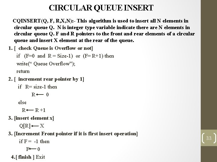
CIRCULAR QUEUE INSERT CQINSERT(Q, F, R, X, N): - This algorithm is used to insert all N elements in circular queue Q. N is integer type variable indicate there are N elements in circular queue Q. F and R pointers to the front and rear elements of a circular queue and insert X element at the rear of the queue. 1. [ check Queue is Overflow or not] if (F=0 and R = Size-1) or (F= R+1) then write(“ Queue Overflow”); return 2. [ increment rear pointer by 1] if R= size-1 then R 0 else R R +1 3. [insert element x] Q[R] X 3. [Increment Front pointer if it is first insert operation] if F = -1 then F 0 4. [ finish ] Exit 33

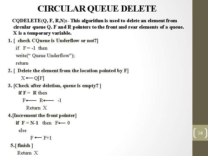
CIRCULAR QUEUE DELETE CQDELETE(Q, F, R, N): - This algorithm is used to delete an element from circular queue Q. F and R pointers to the front and rear elements of a queue. X is a temporary variable. 1. [ check CQueue is Underflow or not? ] if F = -1 then write(“ Queue Underflow”); return 2. [ Delete the element from the location pointed by F] X Q[F] 3. [Check after deletion, queue is empty? ] if F = R then F R -1 Return X 4. [Increment the front pointer] if F = N-1 then F 0 else F F+1 5. [ finish ] Return X 34

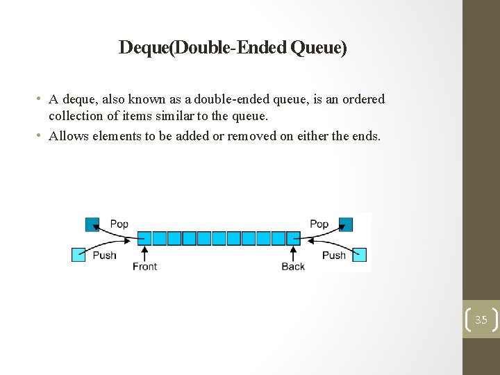
Deque(Double-Ended Queue) • A deque, also known as a double-ended queue, is an ordered collection of items similar to the queue. • Allows elements to be added or removed on either the ends. 35

TYPES OF DEQUE • De. Queue can be represented in two ways : q Input restricted Deque • Elements can be inserted only at one end. • Elements can be removed from both the ends. q Output restricted Deque • Elements can be removed only at one end. • Elements can be inserted from both the ends. 36

Deque as Stack and Queue As STACK • When insertion and deletion is made at the same side. As Queue • When items are inserted at one end and removed at the other end. • This hybrid linear structure provides all the capabilities of stacks and queues in a single data structure. 37

OPERATIONS IN DEQUE • Insert element at right • Insert element at left • Remove element at right 38

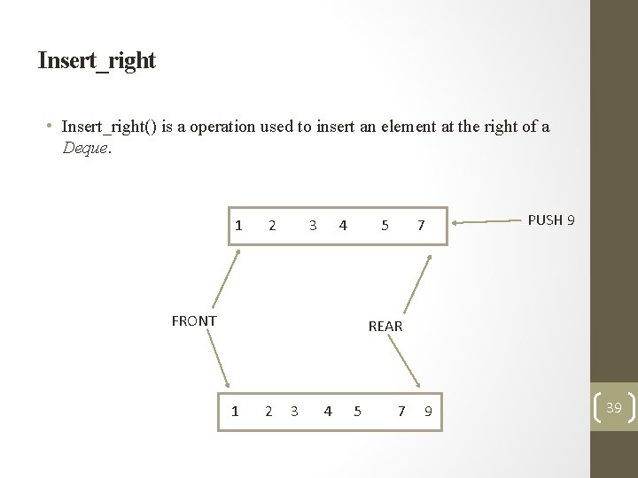
Insert_right • Insert_right() is a operation used to insert an element at the right of a Deque. 1 2 3 4 5 FRONT 7 PUSH 9 REAR 1 2 3 4 5 7 9 39

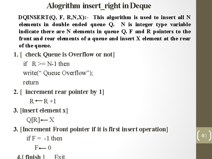
Alogrithm insert_right in Deque DQINSERT(Q, F, R, N, X): - This algorithm is used to insert all N elements in double ended queue Q. N is integer type variable indicate there are N elements in queue Q. F and R pointers to the front and rear elements of a queue and insert X element at the rear of the queue. 1. [ check Queue is Overflow or not] if R >= N-1 then write(“ Queue Overflow”); return 2. [ increment rear pointer by 1] R R +1 3. [insert element x] Q[R] X 3. [Increment Front pointer if it is first insert operation] if F = -1 then F 0 40

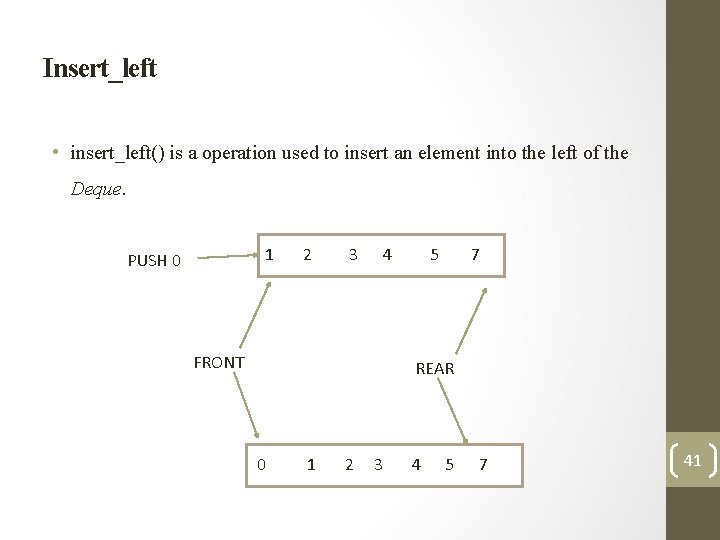
Insert_left • insert_left() is a operation used to insert an element into the left of the Deque. 1 PUSH 0 2 3 4 FRONT 5 7 REAR 0 1 2 3 4 5 7 41

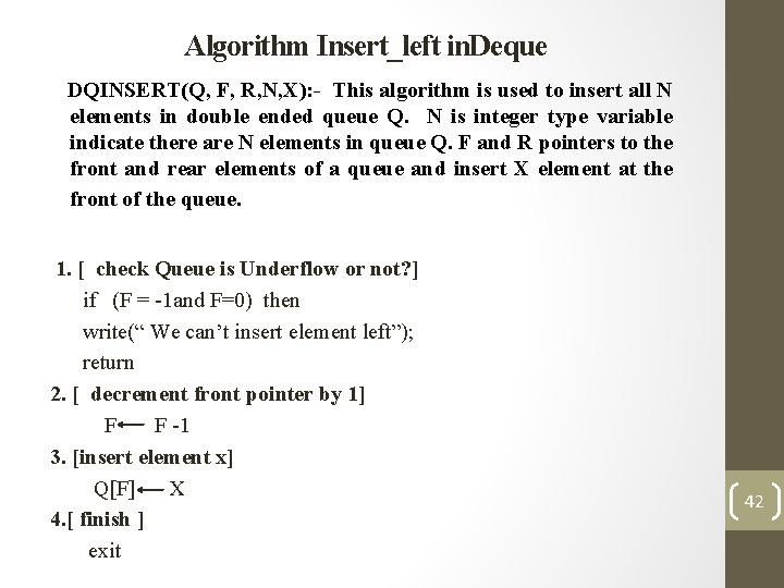
Algorithm Insert_left in. Deque DQINSERT(Q, F, R, N, X): - This algorithm is used to insert all N elements in double ended queue Q. N is integer type variable indicate there are N elements in queue Q. F and R pointers to the front and rear elements of a queue and insert X element at the front of the queue. 1. [ check Queue is Underflow or not? ] if (F = -1 and F=0) then write(“ We can’t insert element left”); return 2. [ decrement front pointer by 1] F F -1 3. [insert element x] Q[F] X 4. [ finish ] exit 42

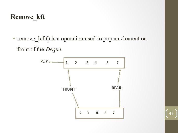
Remove_left • remove_left() is a operation used to pop an element on front of the Deque. POP 1 2 3 4 5 7 REAR FRONT 2 3 4 5 7 43

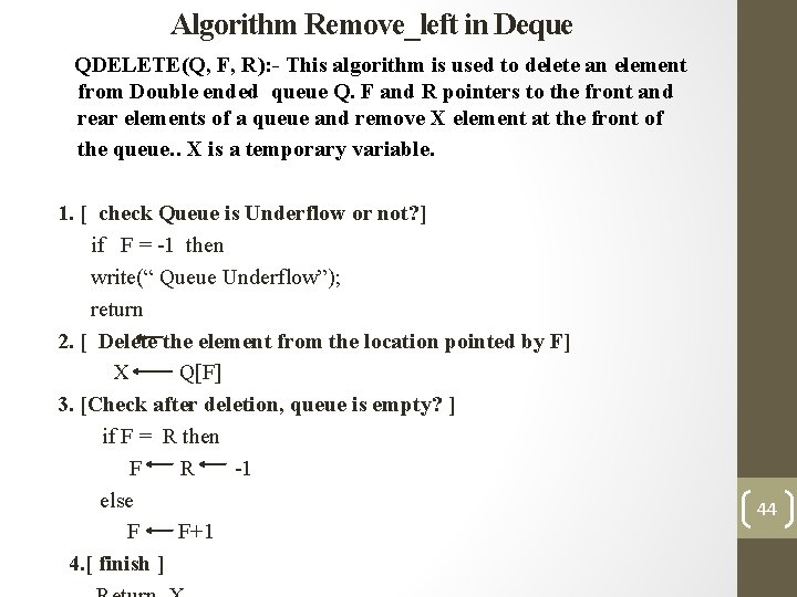
Algorithm Remove_left in Deque QDELETE(Q, F, R): - This algorithm is used to delete an element from Double ended queue Q. F and R pointers to the front and rear elements of a queue and remove X element at the front of the queue. . X is a temporary variable. 1. [ check Queue is Underflow or not? ] if F = -1 then write(“ Queue Underflow”); return 2. [ Delete the element from the location pointed by F] X Q[F] 3. [Check after deletion, queue is empty? ] if F = R then F R -1 else F F+1 4. [ finish ] 44

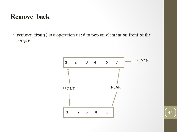
Remove_back • remove_front() is a operation used to pop an element on front of the Deque. 1 2 3 4 5 POP REAR FRONT 1 7 2 3 4 5 45

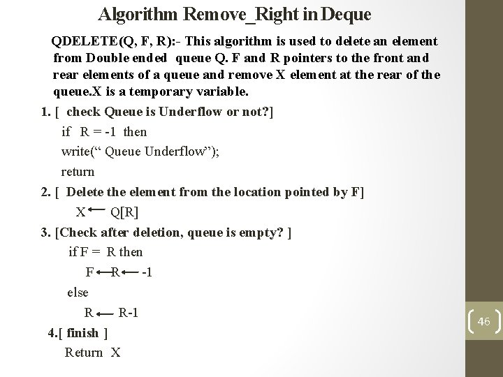
Algorithm Remove_Right in Deque QDELETE(Q, F, R): - This algorithm is used to delete an element from Double ended queue Q. F and R pointers to the front and rear elements of a queue and remove X element at the rear of the queue. X is a temporary variable. 1. [ check Queue is Underflow or not? ] if R = -1 then write(“ Queue Underflow”); return 2. [ Delete the element from the location pointed by F] X Q[R] 3. [Check after deletion, queue is empty? ] if F = R then F R -1 else R R-1 4. [ finish ] Return X 46

Priority Queue • Queues are a standard mechanism for ordering tasks on a first-come, first-served basis • However, some tasks may be more important or timely than others. 47

Applications of Queues • Queues are also very useful in a time-sharing multi-user operating system where many users share the CPU simultaneously. • Whenever a user requests the CPU to run a particular program, the operating system adds the request ( by first of all converting the program into a process that is a running instance of the program, and assigning the process an ID). • This process ID is then added at the end of the queue of jobs waiting to be executed. • Whenever the CPU is free, it executes the job that is at the front of the job queue. 48

Applications of Queues • Similarly, there are queues for shared I/O devices. Each device maintains its own queue of requests. • An example is a print queue on a network printer, which queues up print jobs issued by various users on the network. • The first print request is the first one to be processed. New print requests are added at the end of the queue. 49